Behrens-Fisher

Summary

In this vignette, we introduce the stests R package, which serves as a valuable tool for testing hypotheses related to the Berens-Fisher problem. The package is conveniently hosted on GitHub and is freely accessible for utilization. The core functionality of the stests package revolves around the two_mean_vector_test function. This function generates a specialized R object that allows the use of the standard print function, enabling easy examination of the test results. Furthermore, the two_mean_vector_test function offers the flexibility to generate informative plots showcasing the p-value alongside the corresponding statistics and probabilities. These visualizations provide a comprehensive understanding of the hypothesis testing process, enhancing the interpretability and usability of the stests package. Researchers and practitioners alike can leverage this package to conduct hypothesis testing for the Berens-Fisher problem effectively and efficiently.

Introduction

The multivariate Behrens-Fisher problem deals with testing whether two mean vectors are equal or not based on two random samples obtained from two multivariate normal populations. Symbolically, the Behrens-Fisher problem can be summarized as follows.

Let \(\mathbf{X}_{i1}, \mathbf{X}_{i2}, \ldots, \mathbf{X}_{in_i}\) a random sample from a \(p\)-variate normal population \(N(\boldsymbol{\mu}_i, \boldsymbol{\Sigma}_i)\) with \(i=1, 2\). The Behrens-Fisher problem has the next set of hypothesis.

\[\begin{equation} H_{0}: \boldsymbol{\mu}_1 = \boldsymbol{\mu}_2 \quad \text{vs.} \quad H_{1}: \boldsymbol{\mu}_1 \neq \boldsymbol{\mu}_2 \end{equation}\]

The covariance matrices \(\boldsymbol{\Sigma}_i\) can be unknown and possibly unequal.

Multiple solutions have been proposed to tackle the multivariate Behrens-Fisher problem. The two earliest solutions were given by Bennett (1951) based on the univariate solution of Scheffé (1943) and by James (1954) who extended the univariate Welch series solution.

Yao (1965) proposed an extension of the Welch approximate degrees of freedom and performed a simulation study to compare it with the James solution.

Johansen (1980) presented a solution in the context of general linear models and obtained the exact null distribution of the statistic.

Nel & Van der Merwe (1986) obtained the exact null distribution of the statistic

Kim (1992) presented another extension of the Welch approximate degrees-of-freedom solution by Yao (1965) but using the geometry of confidence ellipsoids for the mean vectors.

Krishnamoorthy & Yu (2004) proposed a new test based on a modification of the solution given by Nel & Van der Merwe (1986).

Gamage, Mathew, & Weerahandi (2004) proposed a procedure for testing equality of the mean vectors using the concept of generalized p-values which are functions of the sufficient statistics.

Yanagihara & Yuan (2005) proposed the F test, the Bartlett correction test and the modified Bartlett correction test.

Kawasaki & Seo (2015) propose an approximate solution to the problem by adjusting the degrees of freedom of the F distribution.

Multivariate statistical tests to compare two mean vectors

In this section we summarize the main multivariate statistical tests reported in the statistical literature for the multivariate Behrens-Fisher problem. For each test we show the statistic and its distribution under the null hypothesis. All tests reported here assume that the underlying distribution is the multivariate normal distribution.

The tests presented below need some inputs as the sample mean vectors

\[\overline{\mathbf{X}}_i = \sum_{j=1}^{n_i} \mathbf{X}_{ij} / n_i \quad \text{with} \quad i=1, 2,\]

and the sample variance-covariance matrices

\[\mathbf{S}_i = \frac{1}{n_i - 1} \sum_{j=1}^{n_i} (\mathbf{X}_{ij} - \overline{\mathbf{X}}_i) (\mathbf{X}_{ij} - \overline{\mathbf{X}}_i)^\top \quad \text{with} \quad i=1, 2.\]

Next are listed the statistical tests to study the hypothesis:

\[\begin{equation} H_{0}: \boldsymbol{\mu}_1 = \boldsymbol{\mu}_2 \quad \text{vs.} \quad H_{1}: \boldsymbol{\mu}_1 \neq \boldsymbol{\mu}_2 \end{equation}\]

Hotelling’s test

This test assumes that \(\mathbf{\Sigma}_1 = \mathbf{\Sigma}_2 = \mathbf{\Sigma}\) but unknow. The statistical test to perform Behrens-Fisher problem is

\[T^2 = \left( \overline{\mathbf{X}}_1 - \overline{\mathbf{X}}_2 \right)^{\top} \left[ \left( \dfrac{1}{n_1} + \dfrac{1}{n_2} \right) \mathbf{S}_p \right] ^{-1} \left( \overline{\mathbf{X}}_1 - \overline{\mathbf{X}}_2 \right), \]

where the pooled variance-covariance matrix \(\mathbf{S}_p\) is given by:

\[\mathbf{S}_p = \dfrac{(n_1 - 1)\; \mathbf{S}_1 + (n_2 - 1)\; \mathbf{S}_2}{n_1 + n_2 - 2}.\]

If \(H_{0}\) is true,

\[T^2 \sim \dfrac{(n_1 + n_2 - 2) \; p}{(n_1 + n_2 - p -1)} \; F_{p, \; n_1 + n_2 - p -1}.\]

First order James’ test (1954)

This test was proposed by without assuming equality of the variance-covariance matrices. The statistical test to perform Behrens-Fisher problem is

\[T^2 = \left( \overline{\mathbf{X}}_1 - \overline{\mathbf{X}}_2 \right) ^{\top} \widetilde{\mathbf{S}} ^{-1} \left( \overline{\mathbf{X}}_1 - \overline{\mathbf{X}}_2 \right),\]

where variance-covariance matrix \(\widetilde{\mathbf{S}}\) is given by:

\[\widetilde{\mathbf{S}} = \widetilde{\mathbf{S}}_1 + \widetilde{\mathbf{S}}_2 = \dfrac{\mathbf{S}_1}{n_1} + \dfrac{\mathbf{S}_2}{n_2} .\]

The critic value (\(cv\)) for this test is given by

\[cv=\chi^2_{\alpha, p} (A + B \chi^2_{\alpha, p}),\]

with

\[\begin{equation*} \label{eq1} \begin{split} A &= 1 + \dfrac{1}{2p}\; \sum _ {i = 1} ^{2} \; \dfrac{\left[ tr\left(\mathbf{ \widetilde{S}} ^{-1} \; \mathbf{\widetilde{S}} _{i}\right) \right] ^{2}}{n_i - 1}, \\ B &= \dfrac{1}{p\;(p+2)}\; \left\lbrace \sum _ {i = 1} ^{2} \; \dfrac{ tr \left[ \left( \mathbf{\widetilde{S}} ^{-1} \; \mathbf{\widetilde{S}} _{i}\right) ^{2} \right]}{n_i - 1} + \dfrac{1}{2}\; \sum _ {i = 1} ^{2} \;\dfrac{\left[ tr\left( \mathbf{\widetilde{S}} ^{-1} \; \mathbf{ \widetilde{S}} _{i}\right) \right] ^{2}}{n_i - 1} \right\rbrace . \end{split} \end{equation*}\]

If \(T^2 > cv\) then the null hypothesis given in Behrens-Fisher problem is rejected.

Yao’s test (1965)

This test was proposed by . The statistical test to perform Behrens-Fisher problem is

\[T^2 = \left( \overline{\mathbf{X}}_1 - \overline{\mathbf{X}}_2 \right) ^{\top} \widetilde{\mathbf{S}} ^{-1} \left( \overline{ \mathbf{X}}_1 - \overline{\mathbf{X}}_2 \right),\]

where the \(\widetilde{\mathbf{S}}\) matrix is given by

\[\widetilde{\mathbf{S}} = \widetilde{\mathbf{S}}_1 + \widetilde{\mathbf{S}}_2 = \dfrac{\mathbf{S}_1}{n_1} + \dfrac{\mathbf{S}_2}{n_2} .\]

If \(H_{0}\) is true,

\[T^2 \sim \dfrac{v\;p}{v-p+1} F _{p,\; v-p+1},\]

where \(v\) is given by

\[v = \left[ \dfrac{1}{n_1-1} \left(\dfrac{ \mathbf{\overline{X}}_{d}^{\top} \;\mathbf{\widetilde{S}}^{-1}\; \mathbf{\widetilde{S}}_{1} \;\mathbf{\widetilde{S}}^{-1}\; \mathbf{\overline{X}} _{d}}{ \mathbf{\overline{X}} _{d}^{\top}\;\mathbf{ \widetilde{S}} ^{-1} \;\mathbf{\overline{X}} _{d}} \right)^{2} + \dfrac{1}{n_2-1} \left( \dfrac{\mathbf{\overline{X}}_{d}^{\top}\; \mathbf{\widetilde{S}} ^{-1}\; \mathbf{\widetilde{S}} _{2} \;\mathbf{\widetilde{S}}^{-1}\; \mathbf{\overline{X}}_{d}}{ \mathbf{\overline{X}} _{d}^{\top} \;\mathbf{\widetilde{S}} ^{-1} \;\mathbf{\overline{X}} _{d}}\right)^{2} \right] ^{-1}, \]

with \(\mathbf{\overline{X}}_{d} = \mathbf{\overline{X}}_{1} -\mathbf{ \overline{X}}_{2}\).

Johansen’s test (1980)

This test was proposed by . The statistical test to perform Behrens-Fisher problem is

\[T^2 = \left( \overline{\mathbf{X}}_1 - \overline{\mathbf{X}}_2 \right) ^{\top} \widetilde{\mathbf{S}} ^{-1} \left( \overline{\mathbf{X}}_1 - \overline{\mathbf{X}}_2 \right),\]

where variance-covariance matrix \(\widetilde{\mathbf{S}}\) is given by:

\[\widetilde{\mathbf{S}} = \widetilde{\mathbf{S}}_1 + \widetilde{\mathbf{S}}_2 = \dfrac{\mathbf{S}_1}{n_1} + \dfrac{\mathbf{S}_2}{n_2}.\]

If \(H_{0}\) is true,

\[T^2 \sim q \, F_{p, v},\]

where

\[q = p + 2D - \dfrac{6D}{p \; (p-1) + 2},\]

\[v = \dfrac{p \; (p+2)}{3D},\]

\[D = \dfrac{1}{2} \; \sum _ {i = 1} ^{2} \; \dfrac{1}{n_i-1} \; \left\lbrace tr \left[ \left(\mathbf{I} - \left( \mathbf{\widetilde{S}}_1 ^{-1} + \mathbf{\widetilde{S}}_2 ^{-1} \right)^{-1} \mathbf{\widetilde{S}}_i ^{-1}\right) ^{2} \right] + \left[ tr \left(\mathbf{I} - \left( \mathbf{\widetilde{S}}_1 ^{-1} +\mathbf{ \widetilde{S}}_2 ^{-1} \right)^{-1}\mathbf{ \widetilde{S}}_i ^{-1}\right) \right]^{2} \right\rbrace .\]

NVM test (1986)

This test was proposed by without assuming equality of the variance-covariance matrices. The statistical test to perform Behrens-Fisher problem is

\[T^2 = \left( \overline{\mathbf{X}}_1 - \overline{\mathbf{X}}_2 \right) ^{\top} \widetilde{\mathbf{S}} ^{-1} \left( \overline{\mathbf{X}}_1 - \overline{\mathbf{X}}_2 \right)\]

where variance-covariance matrix \(\widetilde{\mathbf{S}}\) is given by:

\[\widetilde{\mathbf{S}} = \widetilde{\mathbf{S}}_1 + \widetilde{\mathbf{S}}_2 = \dfrac{\mathbf{S}_1}{n_1} + \dfrac{\mathbf{S}_2}{n_2}\]

If \(H_{0}\) is true,

\[T^2 \sim \dfrac{v\;p}{v-p+1} F _{p, v-p+1}\]

with

\[v = \dfrac{tr \left[ \left( \mathbf{\widetilde{S}} \right)^{2} \right] + \left[ tr \left(\mathbf{ \widetilde{S}} \right) \right]^{2} }{\dfrac{1}{n_1 - 1} \left\lbrace tr \left[ \left( \mathbf{ \widetilde{S}} _{1} \right)^{2} \right] + \left[ tr \left(\mathbf{ \widetilde{S}} _{1} \right) \right]^{2} \right\rbrace + \dfrac{1}{n_2 - 1} \left\lbrace tr \left[ \left(\mathbf{ \widetilde{S}} _{2} \right)^{2} \right] + \left[ tr \left( \mathbf{\widetilde{S}} _{2} \right) \right]^{2} \right\rbrace}\]

Modified NVM test (2004)

This test was proposed by and it is a modification of the test proposed by . The statistical test to perform Behrens-Fisher problem is

\[T^2 = \left( \overline{\mathbf{X}}_1 - \overline{\mathbf{X}}_2 \right) ^{\top} \widetilde{\mathbf{S}} ^{-1} \left( \overline{\mathbf{X}}_1 - \overline{\mathbf{X}}_2 \right)\]

where variance-covariance matrix \(\widetilde{\mathbf{S}}\) is given by:

\[\widetilde{\mathbf{S}} = \widetilde{\mathbf{S}}_1 + \widetilde{\mathbf{S}}_2 = \dfrac{\mathbf{S}_1}{n_1} + \dfrac{\mathbf{S}_2}{n_2}\]

If \(H_{0}\) is true,

\[T^2 \sim \dfrac{v\;p}{v-p+1} F _{p, v-p+1}\]

with

\[v = \dfrac{p + p^2}{\dfrac{1}{n_1-1} \left\lbrace tr \left[ \left( \mathbf{\widetilde{S}} _{1}\; \mathbf{\widetilde{S}} ^{-1} \right)^{2} \right] + \left[ tr \left( \mathbf{\widetilde{S}} _{1}\;\mathbf{ \widetilde{S}} ^{-1} \right) \right]^{2} \right\rbrace + \dfrac{1}{n_2-1} \left\lbrace tr \left[ \left( \mathbf{\widetilde{S}} _{2}\; \mathbf{\widetilde{S}} ^{-1} \right)^{2} \right] + \left[ tr \left( \mathbf{\widetilde{S}} _{2}\;\mathbf{ \widetilde{S}} ^{-1} \right) \right]^{2} \right\rbrace}\]

Gamage’s test (2004)

This test was proposed by . The statistical test to perform Behrens-Fisher problem is

\[T^2 = \left( \overline{\mathbf{X}}_1 - \overline{\mathbf{X}}_2 \right) ^{\top} \widetilde{\mathbf{S}} ^{-1} \left( \overline{\mathbf{X}}_1 - \overline{\mathbf{X}}_2 \right).\]

where variance-covariance matrix \(\widetilde{\mathbf{S}}\) is given by:

\[\widetilde{\mathbf{S}} = \widetilde{\mathbf{S}}_1 + \widetilde{\mathbf{S}}_2 = \dfrac{\mathbf{S}_1}{n_1} + \dfrac{\mathbf{S}_2}{n_2} .\]

If \(t^2\) represents the observed value of \(T^2\), the generalized \(p-\)value for the test is \(P(T_1 \geq t^2 | H_0)\) where the \(T_1\) is a random variable given by

\[\begin{equation} \label{T1} T_1 = \frac{1}{Q_1} \sum_{i=1}^{p} d_i Z_{0i}^2 + \frac{n_2-1}{Q_2} \sum_{i=1}^{p} \left( 1 - \frac{d_i}{n_1-1} \right) d_i Z_{0i}^2. \end{equation}\]

To obtain the generalized \(p-\)value or \(P(T_1 \geq t^2 | H_0)\), we should simulate at least 1000 values from each distribution \(Z_{0i}^2 \sim \chi^2_1\), \(Q_1 \sim \chi^2_{n_1-p}\) and \(Q_2 \sim \chi^2_{n_2-p}\) independently, then those values are replaced in expression of T1 to obtain several \(t_1\), finally, the generalized \(p-\)value is obtained as the percentage rate \(t_1 \geq t^2\).

In expression for T1 the values denoted by \(d_i\) correspond to the eigenvalues of \(\boldsymbol{V}_1\) defined as

\[ \boldsymbol{V}_1 = \frac{n_1-1}{n_1} \left( \frac{\boldsymbol{S}_1}{n_1} + \frac{\boldsymbol{S}_2}{n_2} \right)^{-\frac{1}{2}} \boldsymbol{S}_1 \left( \frac{\boldsymbol{S}_1}{n_1} + \frac{\boldsymbol{S}_2}{n_2} \right)^{-\frac{1}{2}}. \]

For more details about this to test please consult .

Yanagihara and Yuan’s test (2005)

This test was proposed by . The statistical test to perform Behrens-Fisher problem is

\[T^2 = \left( \overline{\mathbf{X}}_1 - \overline{\mathbf{X}}_2 \right) ^{\top} \widetilde{\mathbf{S}} ^{-1} \left( \overline{\mathbf{X}}_1 - \overline{\mathbf{X}}_2 \right).\]

where variance-covariance matrix \(\widetilde{\mathbf{S}}\) is given by:

\[\widetilde{\mathbf{S}} = \widetilde{\mathbf{S}}_1 + \widetilde{\mathbf{S}}_2 = \dfrac{\mathbf{S}_1}{n_1} + \dfrac{\mathbf{S}_2}{n_2} .\]

The null distribution for the statistic \(T^2\) is

\[T^2 \overset{a}{\sim} \dfrac{(n-2) \, p}{n-2-\hat{\theta}_{1}} \, F_{p, \, \hat{v}} ,\]

where the elements \(n\), \(\hat{\theta}_{1}\) and \(\hat{v}\) are defined as follows

\[n = n_1 + n_2\]

\[\hat{\theta}_{1} = \dfrac{p \; \hat{\psi}_{1} + (p-2) \hat{\psi}_{2}}{p \; (p+2)}\]

\[\hat{\theta}_{2} = \dfrac{\hat{\psi}_{1} + 2 \, \hat{\psi}_{2}}{p \, (p+2)} \]

\[\hat{v} = \dfrac{\left( n-2-\hat{\theta}_{1} \right)^2}{(n-2) \, \hat{\theta}_{2} - \hat{\theta}_{1}}\]

\[\overline{\mathbf{S}} = \dfrac{n_2}{n} \; \mathbf{S}_1 + \dfrac{n_1}{n} \; \mathbf{S}_2 \]

\[\hat{\psi}_{1} = \dfrac{n_{2}^{2} \; (n-2)}{n^{2} \; (n_{1}-1)} \; \left\lbrace tr \left( \mathbf{S}_{1} \; \overline{\mathbf{S}}^{-1} \right) \right\rbrace ^2 + \dfrac{n_{1}^{2} \; (n-2)}{n^{2} \; (n_{2}-1)} \; \left\lbrace tr \left( \mathbf{S}_{2} \; \overline{\mathbf{S}}^{-1} \right) \right\rbrace ^2 \]

\[\hat{\psi}_{2} = \dfrac{n_{2}^{2} \; (n-2)}{n^{2} \; (n_{1}-1)} \; \; tr \left( \mathbf{S}_{1} \overline{\mathbf{S}}^{-1} \; \mathbf{S}_{1} \overline{\mathbf{S}}^{-1} \right) + \dfrac{n_{1}^{2} \; (n-2)}{n^{2} \; (n_{2}-1)} \; \; tr \left( \mathbf{S}_{2} \overline{\mathbf{S}}^{-1} \; \mathbf{S}_{2} \overline{\mathbf{S}}^{-1} \right) \]

Bartlett Correction test (2005)

This test was the second test proposed by . The statistical test to perform Behrens-Fisher problem is

\[T^2 = \left( \overline{\mathbf{X}}_1 - \overline{\mathbf{X}}_2 \right) ^{\top} \widetilde{\mathbf{S}} ^{-1} \left( \overline{\mathbf{X}}_1 - \overline{\mathbf{X}}_2 \right).\]

where variance-covariance matrix \(\widetilde{\mathbf{S}}\) is given by:

\[\widetilde{\mathbf{S}} = \widetilde{\mathbf{S}}_1 + \widetilde{\mathbf{S}}_2 = \dfrac{\mathbf{S}_1}{n_1} + \dfrac{\mathbf{S}_2}{n_2} .\]

The null distribution for the statistic \(T^2\) is

\[T^2 \, \sim \, \dfrac{N}{N - \widehat{c}_{1}} \; \; \chi_{p}^{2}\]

where the elements \(N\) and \(\hat{c}_{1}\) are defined as follows

\[N = n_1 + n_2 - 2\]

\[n = n_1 + n_2\]

\[\hat{c}_{1} = \dfrac{\hat{\psi}_{1} + \hat{\psi}_{2}}{p}\]

Modified Bartlett Correction test (2005)

This test was the third test proposed by . The statistical test to perform Behrens-Fisher problem is

\[T^2 = \left( \overline{\mathbf{X}}_1 - \overline{\mathbf{X}}_2 \right) ^{\top} \widetilde{\mathbf{S}} ^{-1} \left( \overline{\mathbf{X}}_1 - \overline{\mathbf{X}}_2 \right).\]

where variance-covariance matrix \(\widetilde{\mathbf{S}}\) is given by:

\[\widetilde{\mathbf{S}} = \widetilde{\mathbf{S}}_1 + \widetilde{\mathbf{S}}_2 = \dfrac{\mathbf{S}_1}{n_1} + \dfrac{\mathbf{S}_2}{n_2} .\]

The null distribution for the statistic \(T^2\) is

\[T^2 \; \sim \; \; N \; \hat{\beta}_{1} \; \left[ \exp \left( \dfrac{\chi_{p}^{2}}{N \; \widehat{\beta}_{1} + \widehat{\beta}_{2}} \right) - 1 \right]\]

where the elements \(N\), \(\hat{\beta}_{1}\) and \(\hat{\beta}_2\) are defined as follows

\[N = n_1 + n_2 - 2\]

\[n = n_1 + n_2\]

\[\hat{\beta}_{1} = \dfrac{2}{\hat{c}_{2} - 2 \; \hat{c}_{1}} = \dfrac{p \; (p+2)}{\hat{\psi}_{1} + 2 \; \hat{\psi}_{2}}\]

\[\hat{\beta}_{2} = \dfrac{(p+2) \; \hat{c}_{2} - 2 \; (p+4) \; \hat{c}_{1}}{2 \; \left( \hat{c}_{2} - 2 \; \hat{c}_{1} \right)} = - \dfrac{(p+2) \; \hat{\psi}_{1}}{2 \; \left( \hat{\psi}_{1} + 2 \; \hat{\psi}_{2} \right)}\]

\[\hat{c}_{1} = \dfrac{\hat{\psi}_{1} + \hat{\psi}_{2}}{p}\]

\[\hat{c}_{2} = \dfrac{2 \; (p+3) \; \widehat{\psi}_{1} + 2 \; (p+4) \; \widehat{\psi}_{2}}{p \; (p+2)}\]

Second Order Procedure (S procedure) test (2015)

This test was the first test proposed by . The statistical test to perform Behrens-Fisher problem is

\[T^2 = \left( \overline{\mathbf{X}}_1 - \overline{\mathbf{X}}_2 \right) ^{\top} \widetilde{\mathbf{S}} ^{-1} \left( \overline{\mathbf{X}}_1 - \overline{\mathbf{X}}_2 \right).\]

where variance-covariance matrix \(\widetilde{\mathbf{S}}\) is given by:

\[\widetilde{\mathbf{S}} = \widetilde{\mathbf{S}}_1 + \widetilde{\mathbf{S}}_2 = \dfrac{\mathbf{S}_1}{n_1} + \dfrac{\mathbf{S}_2}{n_2}.\]

The null distribution for the statistic \(T^2\) is

\[T^2 \; \sim \; \frac{p \, \hat{\phi}_S} {\hat{v}_S} F_{p, \hat{v}_S}\]

where the elements \(\hat{v}_S\) and \(\hat{\phi}_S\) are defined as follows

\[ \hat{v}_S=\frac{2(N^2 - N \theta_1 + \theta_2 - \theta_3)^2}{N^2(N^2-2N\theta_1+2N\theta_4+2\theta_5-\theta_6)-(N^2-N\theta_1+\theta_2-\theta_3)^2}, \]

\[ \hat{\phi}_s = \frac{N^2 \hat{v}_S}{N^2-N\theta_1+\theta_2-\theta_3}, \]

The elements \(\theta_i\) and \(N\) are defined as:

\[\begin{align*} n &= n_1 + n_2, \\ N &= n - 2 \end{align*}\]

\[ \theta_1 = \frac{1}{p(p+2)} \sum_{i=1}^{2} c_i \left[ p \left( a_i^{(1)} \right)^2 + (p-2) a_i^{(2)} \right], \]

\[ \theta_2 = \frac{1}{p(p+2)(p+4)} \sum_{i=1}^{2} d_i \left[ 4 p^2 a_i^{(3)} + (p-2)(3p+4) a_i^{(1)} a_i^{(2)} + p(p+2) \left( a_i^{(1)} \right)^3 \right], \]

\[\begin{align*} \theta_3 &= \frac{1}{p(p+2)(p+4)(p+6)} \left\lbrace \sum_{i=1}^{2} c_i^2 \left[ p^2(5p+14) a_i^{(4)} + 4(p+3)(p+2)(p-2) a_i^{(1)} a_i^{(3)} \right. \right. \\ &+ \left. \left. p(p+3)(p-2) \left( a_i^{(2)} \right)^2 + 2(p^3+5p^2+7p+6) a_i^{(2)} \left( a_i^{(1)} \right)^2 -p(p+4) \left(a_i^{(1)}\right)^4 \right] \right. \\ &+ \left. 4 (p+3)(p+2)(p-2)\psi_1 + 4p(p+2)(p-2)\psi_2 + 4p(p+4)(p+2)\psi_3 \right. \\ &- \left. 2p(p-2)\psi_4-2(p+3)(p-2)\psi_5+2p(p+4)(p-2)\psi_6-2p(p+4)\psi_7+2p(p+4)(3p+2)\psi_8 \right\rbrace, \end{align*}\]

\[ \theta_4 = \frac{1}{p(p+2)} \sum_{i=1}^{2} c_i \left[ \left( a_i^{(1)} \right)^2 + 2a_i^{(2)} \right], \]

\[ \theta_5 = \frac{1}{p(p+2)(p+4)} \sum_{i=1}^{2} d_i \left[ 4(p^2-3p+4)a_i^{(3)} + 3p(p-4)a_i^{(1)}a_i^{(2)} + p^2 \left(a_i^{(1)}\right)^3 \right], \]

\[\begin{align*} \theta_6 &= \frac{1}{p(p+2)(p+4)(p+6)} \left[ \sum_{i=1}^{2} c_i^2 \left[ 2(p+1)(5p^2-14p+24)a_i^{(4)} \right. \right. \\ &+ \left. \left. 4(p-4)(2p^2+5p+6)a_i^{(1)}a_i^{(3)} + (p-2)(p-4)(2p+3)\left(a_i^{(2)}\right)^2 \right. \right. \\ &+ \left. \left. 2(p+2)(2p^2-p+12)a_i^{(2)}\left(a_i^{(1)}\right)^2 - 3(p^2+2p-4)\left(a_i^{(1)}\right)^4 \right] \right. \\ &+ \left. 4(p-4)(2p^2+5p+6)\psi_1 + 8p(p-2)(p-4)\psi_2 + 8p(p^2+4p+2)\psi_3 \right. \\ &- \left. 4(p-2)(p-4)\psi_4 - 6(p-4)(p+2)\psi_5 + 4(p+3)(p-2)(p-4)\psi_6 \right. \\ &- \left. 6(p^2+2p-4)\psi_7 + 12(p^3+p^2-2p+8)\psi_8 \right], \end{align*}\]

\[\begin{align*} a_i^{(l)} &= tr \left( \Sigma_i \bar{\Sigma}^{-1} \right)^l, \, \text{for} \, i=1, 2, \, \text{and} \, l=1, 2, 3, 4, \\ b^{(q, r, s)} &= tr \left[ \left(\Sigma_1 \bar{\Sigma}^{-1}\right)^q \left(\Sigma_2 \bar{\Sigma}^{-1}\right)^r \right]^s \\ c_i &= \frac{(n-n_i)^2(n-2)}{n^2(n_i-1)}, \\ d_i &= \frac{(n-n_i)^3(n-2)^2}{n^3(n_i-1)^2} \\ (q, r, s) &= (1,1,1), (1,1,2), (1,2,1), (2,1,1), (2,2,1). \end{align*}\]

\[\begin{align*} \psi_1 &= c_1 c_2 \left( a_1^{(1)} b^{(1,2,1)} + a_2^{(1)} b^{(2,1,1)} \right), & \psi_2 &= c_1 c_2 b^{(2,2,1)}, \\ \psi_3 &= c_1 c_2 a_1^{(1)} a_2^{(1)} b^{(1,1,1)}, & \psi_4 &= c_1 c_2 a_1^{(2)} a_2^{(2)}, \\ \psi_5 &= c_1 c_2 \left( a_1^{(2)} \left(a_2^{(1)}\right)^2 + \left(a_1^{(1)}\right)^2 a_2^{(2)} \right), & \psi_6 &= c_1 c_2 \left( b^{(1,1,1)} \right)^2, \\ \psi_7 &= c_1 c_2 \left(a_1^{(1)}\right)^2 \left(a_2^{(1)}\right)^2, & \psi_8 &= c_1 c_2 b^{(1,1,2)} \end{align*}\]

Bias Correction Procedure (BC Procedure) test (2015)

This test was the second test proposed by . The statistical test to perform Behrens-Fisher problem is

\[T^2 = \left( \overline{\mathbf{X}}_1 - \overline{\mathbf{X}}_2 \right) ^{\top} \widetilde{\mathbf{S}} ^{-1} \left( \overline{\mathbf{X}}_1 - \overline{\mathbf{X}}_2 \right).\]

where variance-covariance matrix \(\widetilde{\mathbf{S}}\) is given by:

\[\widetilde{\mathbf{S}} = \widetilde{\mathbf{S}}_1 + \widetilde{\mathbf{S}}_2 = \dfrac{\mathbf{S}_1}{n_1} + \dfrac{\mathbf{S}_2}{n_2}.\]

The null distribution for the statistic \(T^2\) is

\[T^2 \; \sim \; \frac{p \, \hat{\phi}_{BC}} {\hat{v}_{BC}} F_{p, \hat{v}_{BC}}\]

where the elements \(\hat{v}_{BC}\) and \(\hat{\phi}_{BC}\) are defined as follows

\[ \hat{v}_{BC}=\frac{2(N^2 - N \theta_1 + \theta_2 - \theta_3 - \theta_1^\star)^2}{N^2(N^2-2N\theta_1+2N\theta_4+2\theta_5-\theta_6-2\theta_1^\star+2\theta_4^\star)-(N^2-N\theta_1+\theta_2-\theta_3-\theta_1^\star)^2}, \]

\[ \hat{\phi}_{BC} = \frac{N^2 \hat{v}_{BC}}{N^2-N\theta_1+\theta_2-\theta_3-\theta_1^\star}, \]

The elements \(\theta_i\) are defined by the same expressions defined in the Second Order Procedure (S procedure) test whereas the elements \(\theta_1^\star\) and \(\theta_4^\star\) are given by

\[ \theta_1^\star = \eta_1 - \eta_2 + \eta_3, \quad \theta_4^\star = \eta_4 - \eta_5 + \eta_6. \]

stests package

stests is an useful package in which are implemented several statistical tests for multivariate analysis. The current version of the package is hosted in github and any user could download the package using the next code.

if (!require('devtools')) install.packages('devtools')
devtools::install_github('fhernanb/stests', force=TRUE)

To use the package we can use the usual way.

library(stests)

two_mean_vector_test is the main function in the stests package to perform tests for the multivariate Behrens-Fisher problem. The function deals with summarized data, this means that the user should provide the sample means \(\overline{\mathbf{X}}_1\), \(\overline{\mathbf{X}}_2\), the sample variances \(\mathbf{S}_1\), \(\mathbf{S}_2\), and the sample sizes \(n_1\) and \(n_2\).

two_mean_vector_test(xbar1, s1, n1, xbar2, s2, n2, 
                     method="T2", alpha=0.05)

In the next section, we present examples to illustrate the function use.

Examples

In this section we present some examples of the two_mean_vector_test( ) function.

Hotelling’s test

The data correspond to the example 5.4.2 from page 137. The objective is to test the hypothesis \(H_{0}: \boldsymbol{\mu}_1 = \boldsymbol{\mu}_2\) versus \(H_{1}: \boldsymbol{\mu}_1 \neq \boldsymbol{\mu}_2\).

Next are the input data to perform the test.

n1 <- 32
xbar1 <- c(15.97, 15.91, 27.19, 22.75)
s1 <- matrix(c(5.192, 4.545, 6.522, 5.25, 
               4.545, 13.18, 6.76, 6.266, 
               6.522, 6.76, 28.67, 14.47, 
               5.25, 6.266, 14.47, 16.65), ncol=4)

n2 <- 32
xbar2 <- c(12.34, 13.91, 16.66, 21.94)
s2 <- matrix(c(9.136, 7.549, 4.864, 4.151, 
               7.549, 18.6, 10.22, 5.446, 
               4.864, 10.22, 30.04, 13.49, 
               4.151, 5.446, 13.49, 28), ncol=4)

To perform the test we use the two_mean_vector_test function using method="T2" as follows.

res <- two_mean_vector_test(xbar1=xbar1, s1=s1, n1=n1,
                            xbar2=xbar2, s2=s2, n2=n2, 
                            method="T2")
res
## 
##  T2 test for two mean vectors
## 
## data:  this test uses summarized data
## T2 = 97.678, F = 23.238, df1 = 4, df2 = 59, p-value = 1.444e-11
## alternative hypothesis: mu1 is not equal to mu2 
## 
## sample estimates:
##        Sample 1 Sample 2
## xbar_1    15.97    12.34
## xbar_2    15.91    13.91
## xbar_3    27.19    16.66
## xbar_4    22.75    21.94

We can depict the \(p-\)value as follows.

plot(res, from=20, to=25, shade.col="tomato")

First order James’ test

The data correspond to the example in page 41 from . The objective is to test the hypothesis \(H_{0}: \boldsymbol{\mu}_1 = \boldsymbol{\mu}_2\) versus \(H_{1}: \boldsymbol{\mu}_1 \neq \boldsymbol{\mu}_2\).

Next are the input data to perform the test.

n1 <- 16
xbar1 <- c(9.82, 15.06)
s1 <- matrix(c(120, -16.3,
               -16.3, 17.8), ncol=2)

n2 <- 11
xbar2 <- c(13.05, 22.57)
s2 <- matrix(c(81.8, 32.1,
               32.1, 53.8), ncol=2)

To perform the test we use the two_mean_vector_test function using method="james" with significance level alpha=0.05 as follows.

res <- two_mean_vector_test(xbar1=xbar1, s1=s1, n1=n1,
                            xbar2=xbar2, s2=s2, n2=n2,
                            method="james", alpha=0.05)
res
## 
##  James test for two mean vectors
## 
## data:  this test uses summarized data
## T2 = 9.4455, critic_value = 7.2308, df = 2
## alternative hypothesis: mu1 is not equal to mu2 
## 
## sample estimates:
##        Sample 1 Sample 2
## xbar_1     9.82    13.05
## xbar_2    15.06    22.57

We can depict the \(p-\)value as follows.

plot(res, from=5, to=10, shade.col="lightgreen")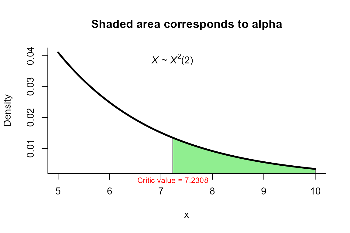

Yao’s test

The data correspond to the example in page 141 from . The objective is to test the hypothesis \(H_{0}: \boldsymbol{\mu}_1 = \boldsymbol{\mu}_2\) versus \(H_{1}: \boldsymbol{\mu}_1 \neq \boldsymbol{\mu}_2\).

Next are the input data to perform the test.

n1 <- 16
xbar1 <- c(9.82, 15.06)
s1 <- matrix(c(120, -16.3,
               -16.3, 17.8), ncol=2)

n2 <- 11
xbar2 <- c(13.05, 22.57)
s2 <- matrix(c(81.8, 32.1,
               32.1, 53.8), ncol=2)

To perform the test we use the two_mean_vector_test function using method="yao" as follows.

res <- two_mean_vector_test(xbar1=xbar1, s1=s1, n1=n1,
                            xbar2=xbar2, s2=s2, n2=n2,
                            method="yao")
res
## 
##  Yao test for two mean vectors
## 
## data:  this test uses summarized data
## T2 = 9.4455, F = 4.3855, df1 = 2.000, df2 = 13.001, p-value = 0.03503
## alternative hypothesis: mu1 is not equal to mu2 
## 
## sample estimates:
##        Sample 1 Sample 2
## xbar_1     9.82    13.05
## xbar_2    15.06    22.57

We can depict the \(p-\)value as follows.

plot(res, from=2, to=6, shade.col="pink")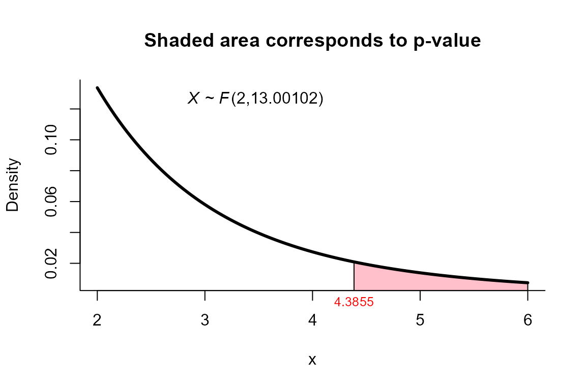

Johansen’s test

For this example we use the same dataset described in the example for Yao’s test but using the method="johansen" as follows.

Next are the input data to perform the test.

n1 <- 16
xbar1 <- c(9.82, 15.06)
s1 <- matrix(c(120, -16.3,
               -16.3, 17.8), ncol=2)

n2 <- 11
xbar2 <- c(13.05, 22.57)
s2 <- matrix(c(81.8, 32.1,
               32.1, 53.8), ncol=2)

To perform the test we use the two_mean_vector_test function using method="johansen" as follows.

res <- two_mean_vector_test(xbar1=xbar1, s1=s1, n1=n1,
                            xbar2=xbar2, s2=s2, n2=n2,
                            method="johansen")
res
## 
##  Johansen test for two mean vectors
## 
## data:  this test uses summarized data
## T2 = 9.4455, F = 4.5476, df1 = 2.000, df2 = 16.309, p-value = 0.02587
## alternative hypothesis: mu1 is not equal to mu2 
## 
## sample estimates:
##        Sample 1 Sample 2
## xbar_1     9.82    13.05
## xbar_2    15.06    22.57

We can depict the \(p-\)value as follows.

plot(res, from=2, to=6, shade.col="aquamarine1")

NVM test

The data correspond to the example 4.1 from page 3729. The objective is to test the hypothesis \(H_{0}: \boldsymbol{\mu}_1 = \boldsymbol{\mu}_2\) versus \(H_{1}: \boldsymbol{\mu}_1 \neq \boldsymbol{\mu}_2\).

Next are the input data to perform the test.

n1 <- 45
xbar1 <- c(204.4, 556.6)
s1 <- matrix(c(13825.3, 23823.4,
               23823.4, 73107.4), ncol=2)

n2 <- 55
xbar2 <- c(130.0, 355.0)
s2 <- matrix(c(8632.0, 19616.7,
               19616.7, 55964.5), ncol=2)

To perform the test we use the two_mean_vector_test function using method="nvm" as follows.

res <- two_mean_vector_test(xbar1=xbar1, s1=s1, n1=n1,
                            xbar2=xbar2, s2=s2, n2=n2,
                            method="nvm")
res
## 
##  Nel and Van der Merwe test for two mean vectors
## 
## data:  this test uses summarized data
## T2 = 15.6585, F = 7.7402, df1 = 2.000, df2 = 86.873, p-value =
## 0.0008064
## alternative hypothesis: mu1 is not equal to mu2 
## 
## sample estimates:
##        Sample 1 Sample 2
## xbar_1    204.4      130
## xbar_2    556.6      355

We can depict the \(p-\)value as follows.

plot(res, from=6, to=10, shade.col="cyan2")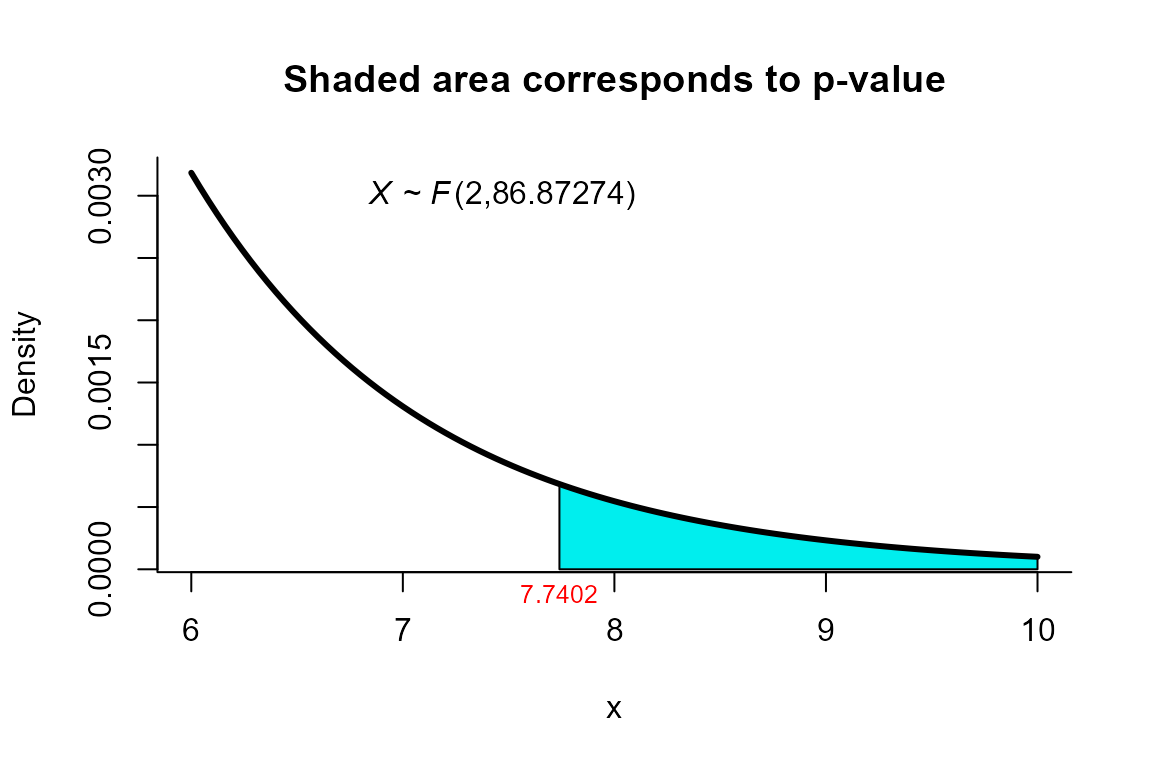

Modified NVM test

For this example we use the same dataset described in the example for NVM test but using the method="mnvn" as follows.

Next are the input data to perform the test.

n1 <- 45
xbar1 <- c(204.4, 556.6)
s1 <- matrix(c(13825.3, 23823.4,
               23823.4, 73107.4), ncol=2)

n2 <- 55
xbar2 <- c(130.0, 355.0)
s2 <- matrix(c(8632.0, 19616.7,
               19616.7, 55964.5), ncol=2)

To perform the test we use the two_mean_vector_test function using method="mnvm" as follows.

res <- two_mean_vector_test(xbar1=xbar1, s1=s1, n1=n1,
                            xbar2=xbar2, s2=s2, n2=n2,
                            method="mnvm")
res
## 
##  Modified Nel and Van der Merwe test for two mean vectors
## 
## data:  this test uses summarized data
## T2 = 15.6585, F = 7.7261, df1 = 2.000, df2 = 74.906, p-value = 0.00089
## alternative hypothesis: mu1 is not equal to mu2 
## 
## sample estimates:
##        Sample 1 Sample 2
## xbar_1    204.4      130
## xbar_2    556.6      355

We can depict the \(p-\)value as follows.

plot(res, from=6, to=10, shade.col="lightgoldenrodyellow")

Gamage’s test

For this example we use the same dataset described in the example for NVM test but using the method="gamage" as follows.

Next are the input data to perform the test.

n1 <- 45
xbar1 <- c(204.4, 556.6)
s1 <- matrix(c(13825.3, 23823.4,
               23823.4, 73107.4), ncol=2)

n2 <- 55
xbar2 <- c(130.0, 355.0)
s2 <- matrix(c(8632.0, 19616.7,
               19616.7, 55964.5), ncol=2)

To perform the test we use the two_mean_vector_test function using method="gamage" as follows.

res <- two_mean_vector_test(xbar1=xbar1, s1=s1, n1=n1,
                            xbar2=xbar2, s2=s2, n2=n2,
                            method="gamage")
res
## 
##  Gamage test for two mean vectors
## 
## data:  this test uses summarized data
## T2 = 15.659, p-value = 0.001
## alternative hypothesis: mu1 is not equal to mu2 
## 
## sample estimates:
##        Sample 1 Sample 2
## xbar_1    204.4      130
## xbar_2    556.6      355

We can depict the \(p-\)value as follows.

plot(res, from=0, to=20, shade.col="lightgoldenrodyellow")

Yanagihara and Yuan’s test

For this example we use the same dataset described in the example for NVM test but using the method="yy" as follows.

Next are the input data to perform the test.

n1 <- 45
xbar1 <- c(204.4, 556.6)
s1 <- matrix(c(13825.3, 23823.4,
               23823.4, 73107.4), ncol=2)

n2 <- 55
xbar2 <- c(130.0, 355.0)
s2 <- matrix(c(8632.0, 19616.7,
               19616.7, 55964.5), ncol=2)

To perform the test we use the two_mean_vector_test function using method="yy" as follows.

res <- two_mean_vector_test(xbar1=xbar1, s1=s1, n1=n1,
                            xbar2=xbar2, s2=s2, n2=n2,
                            method="yy")
res
## 
##  Yanagihara and Yuan test for two mean vectors
## 
## data:  this test uses summarized data
## T2 = 15.6585, F = 7.7272, df1 = 2.000, df2 = 74.309, p-value =
## 0.0008937
## alternative hypothesis: mu1 is not equal to mu2 
## 
## sample estimates:
##        Sample 1 Sample 2
## xbar_1    204.4      130
## xbar_2    556.6      355

We can depict the \(p-\)value as follows.

plot(res, from=6, to=10, shade.col='gold2')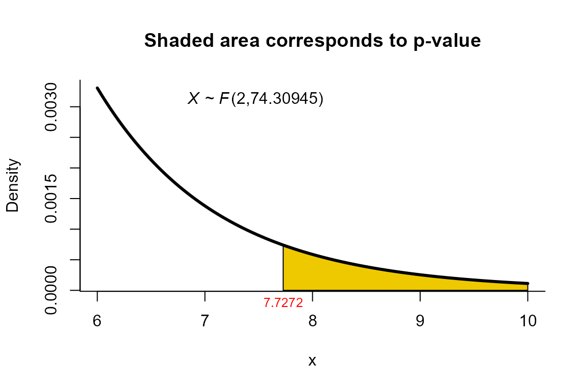

Bartlett Correction test

For this example we use the same dataset described in the example for NVM test but using the method="byy" as follows.

Next are the input data to perform the test.

n1 <- 45
xbar1 <- c(204.4, 556.6)
s1 <- matrix(c(13825.3, 23823.4,
               23823.4, 73107.4), ncol=2)

n2 <- 55
xbar2 <- c(130.0, 355.0)
s2 <- matrix(c(8632.0, 19616.7,
               19616.7, 55964.5), ncol=2)

To perform the test we use the two_mean_vector_test function using method="byy" as follows.

res <- two_mean_vector_test(xbar1=xbar1, s1=s1, n1=n1,
                            xbar2=xbar2, s2=s2, n2=n2,
                            method="byy")
res
## 
##  Bartlett Correction test for two mean vectors
## 
## data:  this test uses summarized data
## T2 = 15.659, X-squared = 15.040, df = 2, p-value = 0.0005422
## alternative hypothesis: mu1 is not equal to mu2 
## 
## sample estimates:
##        Sample 1 Sample 2
## xbar_1    204.4      130
## xbar_2    556.6      355

We can depict the \(p-\)value as follows.

plot(res, from=12, to=20, shade.col='hotpink2')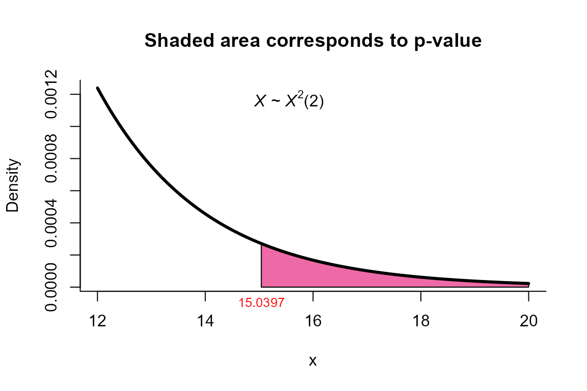

Modified Bartlett Correction test

For this example we use the same dataset described in the example for NVM test but using the method="mbyy" as follows.

Next are the input data to perform the test.

n1 <- 45
xbar1 <- c(204.4, 556.6)
s1 <- matrix(c(13825.3, 23823.4,
               23823.4, 73107.4), ncol=2)

n2 <- 55
xbar2 <- c(130.0, 355.0)
s2 <- matrix(c(8632.0, 19616.7,
               19616.7, 55964.5), ncol=2)

To perform the test we use the two_mean_vector_test function using method="mbyy" as follows.

res <- two_mean_vector_test(xbar1=xbar1, s1=s1, n1=n1,
                            xbar2=xbar2, s2=s2, n2=n2,
                            method="mbyy")
res
## 
##  Modified Bartlett Correction test for two mean vectors
## 
## data:  this test uses summarized data
## T2 = 15.659, X-squared = 14.044, df = 2, p-value = 0.000892
## alternative hypothesis: mu1 is not equal to mu2 
## 
## sample estimates:
##        Sample 1 Sample 2
## xbar_1    204.4      130
## xbar_2    556.6      355

We can depict the \(p-\)value as follows.

plot(res, from=12, to=20, shade.col='green3')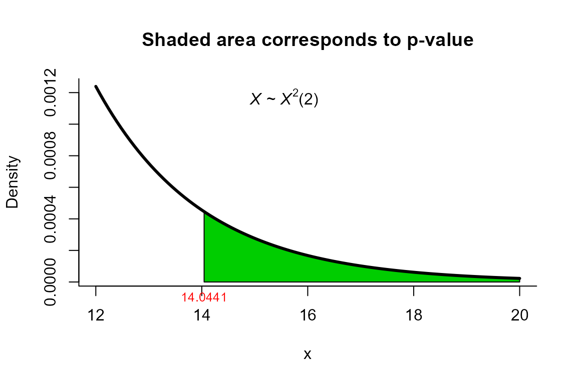

Second Order Procedure (S procedure) test

For this example we use the same dataset described in the example for NVM test but using the method="ks1" as follows.

Next are the input data to perform the test.

n1 <- 45
xbar1 <- c(204.4, 556.6)
s1 <- matrix(c(13825.3, 23823.4,
               23823.4, 73107.4), ncol=2)

n2 <- 55
xbar2 <- c(130.0, 355.0)
s2 <- matrix(c(8632.0, 19616.7,
               19616.7, 55964.5), ncol=2)

To perform the test we use the two_mean_vector_test function using method="ks1" as follows.

res <- two_mean_vector_test(xbar1=xbar1, s1=s1, n1=n1,
                            xbar2=xbar2, s2=s2, n2=n2,
                            method="ks1")
res
## 
##  Kawasaki and Seo (Second order) test for two mean vectors
## 
## data:  this test uses summarized data
## T2 = 15.6585, F = 7.7247, df1 = 2.000, df2 = 49.576, p-value = 0.001201
## alternative hypothesis: mu1 is not equal to mu2 
## 
## sample estimates:
##        Sample 1 Sample 2
## xbar_1    204.4      130
## xbar_2    556.6      355

We can depict the \(p-\)value as follows.

plot(res, from=6, to=10, shade.col='hotpink1')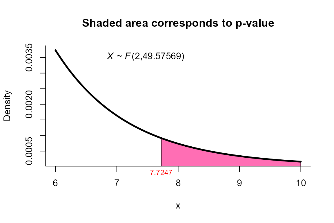

Bias Correction Procedure (BC Procedure) test

For this example we use the same dataset described in the example for NVM test but using the method="ks2" as follows.

Next are the input data to perform the test.

n1 <- 45
xbar1 <- c(204.4, 556.6)
s1 <- matrix(c(13825.3, 23823.4,
               23823.4, 73107.4), ncol=2)

n2 <- 55
xbar2 <- c(130.0, 355.0)
s2 <- matrix(c(8632.0, 19616.7,
               19616.7, 55964.5), ncol=2)

To perform the test we use the two_mean_vector_test function using method="ks2" as follows.

res <- two_mean_vector_test(xbar1=xbar1, s1=s1, n1=n1,
                            xbar2=xbar2, s2=s2, n2=n2,
                            method="ks2")
res
## 
##  Kawasaki and Seo (Bias Correction) test for two mean vectors
## 
## data:  this test uses summarized data
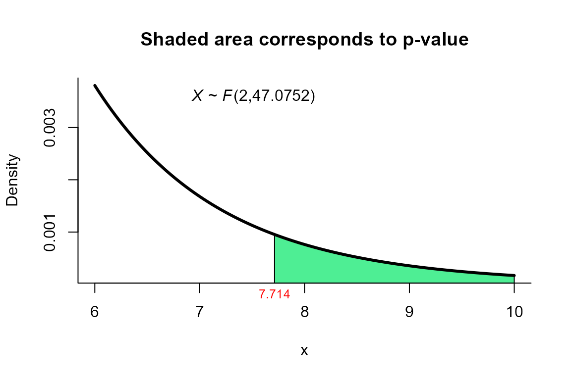
## T2 = 15.659, F = 7.714, df1 = 2.000, df2 = 47.075, p-value = 0.001266
## alternative hypothesis: mu1 is not equal to mu2 
## 
## sample estimates:
##        Sample 1 Sample 2
## xbar_1    204.4      130
## xbar_2    556.6      355

We can depict the \(p-\)value as follows.

plot(res, from=6, to=10, shade.col='seagreen2')

References

Bennett, B. M. (1951). Note on a solution of the generalized behrens–fisher problem. Ann. Inst. Statist. Math., 2, 87–90.

Gamage, J., Mathew, T., & Weerahandi, S. (2004). Generalized p-values and generalized confidence regions for the multivariate behrens–fisher problem and MANOVA. Journal of Multivariate Analysis, 88, 177–189.

James, G. (1954). Tests of linear hypotheses in univariate and multivariate analysis when the ratios of the population variances are unknown. Biometrika, 41, 19–43. [Oxford University Press, Biometrika Trust].

Johansen, S. (1980). The welch-james approximation to the distribution of the residual sum of squares in a weighted linear regression. Biometrika, 67(1), 85–92.

Kawasaki, T., & Seo, T. (2015). A two sample test for mean vectors with unequal covariance matrices. Communications in Statistics - Simulation and Computations, 44, 1850–1866.

Kim, S.-J. (1992). A practical solution to the multivariate behrens-fisher problem. Biometrika, 79(1), 171–176. [Oxford University Press, Biometrika Trust]. Retrieved from http://www.jstor.org/stable/2337157

Krishnamoorthy, K., & Yu, J. (2004). Modified nel and van der merwe test for the multivariate behrens–fisher problem. Statistics & Probability Letters, 66(2), 161–169.

Nel, D. G., & Van der Merwe, C. A. (1986). A solution to the multivariate behrens-fisher problem. Communications in Statistics - Theory and Methods, 15(12), 3719–3735.

Scheffé, H. (1943). On solutions of the behrens-fisher problem, based on the t-distribution. The Annals of Mathematical Statistics, 14(1), 35–44. Institute of Mathematical Statistics. Retrieved from http://www.jstor.org/stable/2236000

Yanagihara, H., & Yuan, K. (2005). Three approximate solutions to the multivariate behrens-fisher problem. Communications in Statistics - Simulation and Computations, 34, 975–988.

Yao, Y. (1965). An approximate degrees of freedom solution to the multivariate beherens-fisher problem. Biometrika, 52(1/2), 139–147.

Freddy Hernandez and Jean Paul Piedrahita

2023-08-01

Summary

Introduction

Multivariate statistical tests to compare two mean vectors

Hotelling’s test

First order James’ test (1954)

Yao’s test (1965)

Johansen’s test (1980)

NVM test (1986)

Modified NVM test (2004)

Gamage’s test (2004)

Yanagihara and Yuan’s test (2005)

Bartlett Correction test (2005)

Modified Bartlett Correction test (2005)

Second Order Procedure (S procedure) test (2015)

Bias Correction Procedure (BC Procedure) test (2015)

stests package

Examples

Hotelling’s test

First order James’ test

Yao’s test

Johansen’s test

NVM test

Modified NVM test

Gamage’s test

Yanagihara and Yuan’s test

Bartlett Correction test

Modified Bartlett Correction test

Second Order Procedure (S procedure) test

Bias Correction Procedure (BC Procedure) test

References