Tests for Equality of Two Normal Mean Vectors
Source:R/two_mean_vector_test.R
two_mean_vector_test.RdThe function implements the test for \(H_0: \mu_1 = \mu_2\) versus \(H_1: \mu_1\) not = \(\mu_2\) when two random samples are obtained from two p-variate normal populations \(Np(\mu_1, \Sigma_1)\) and \(Np(\mu_2, \Sigma_2)\) respectively. By default, the function performs the Hotelling test for two normal mean vectors assumming equality in the covariance matrices. Other tests for the multivariate Behrens-Fisher problem are also implemented, see the argument method below.
two_mean_vector_test(
  xbar1,
  s1,
  n1,
  xbar2,
  s2,
  n2,
  delta0 = NULL,
  method = "T2",
  alpha = 0.05
)
Arguments
- xbar1
a vector with the sample mean from population 1.
- s1
a matrix with sample variances and covariances from population 1.
- n1
sample size 1.
- xbar2
a vector with the sample mean from population 2.
- s2
a matrix with sample variances and covariances from population 2.
- n2
sample size 2.
- delta0
a number indicating the true value of the difference in means.
- method
a character string specifying the method,
"T2"(default),"james"(James' first order test), please see the details section for other methods.- alpha
the significance level only for method
"james", by default its value is 0.05.
Value
A list with class "htest" containing the following components:
- statistic
the value of the statistic.
- parameter
the degrees of freedom for the test.
- p.value
the p-value for the test.
- estimate
the estimated mean vectors.
- method
a character string indicating the type of test performed.
Details
the "method" argument must be one of
"T2" (default),
"james" (James' first order test),
"yao" (Yao's test),
"johansen" (Johansen's test),
"nvm" (Nel and Van der Merwe test),
"mnvm" (modified Nel and Van der Merwe test),
"gamage" (Gamage's test),
"yy" (Yanagihara and Yuan test),
"byy" (Bartlett Correction test),
"mbyy" (modified Bartlett Correction test),
"ks1" (Second Order Procedure),
"ks2" (Bias Correction Procedure).
For James test the critic value is reported, we reject \(H_0\) if T2 > critic_value.
Examples
# Example 5.4.2 from Rencher & Christensen (2012) page 137,
# using Hotelling's test
n1 <- 32
xbar1 <- c(15.97, 15.91, 27.19, 22.75)
s1 <- matrix(c(5.192, 4.545, 6.522, 5.25,
4.545, 13.18, 6.76, 6.266,
6.522, 6.76, 28.67, 14.47,
5.25, 6.266, 14.47, 16.65), ncol = 4)
n2 <- 32
xbar2 <- c(12.34, 13.91, 16.66, 21.94)
s2 <- matrix(c(9.136, 7.549, 4.864, 4.151,
7.549, 18.6, 10.22, 5.446,
4.864, 10.22, 30.04, 13.49,
4.151, 5.446, 13.49, 28), ncol = 4)
res1 <- two_mean_vector_test(xbar1 = xbar1, s1 = s1, n1 = n1,
xbar2 = xbar2, s2 = s2, n2 = n2,
method = "T2")
res1
#>
#> T2 test for two mean vectors
#>
#> data: this test uses summarized data
#> T2 = 97.678, F = 23.238, df1 = 4, df2 = 59, p-value = 1.444e-11
#> alternative hypothesis: mu1 is not equal to mu2
#>
#> sample estimates:
#> Sample 1 Sample 2
#> xbar_1 15.97 12.34
#> xbar_2 15.91 13.91
#> xbar_3 27.19 16.66
#> xbar_4 22.75 21.94
#>
plot(res1, from=21, to=25, shade.col='tomato')
 # Example 3.7 from Seber (1984) page 116.
# using the James first order test (1954).
n1 <- 16
xbar1 <- c(9.82, 15.06)
s1 <- matrix(c(120, -16.3,
-16.3, 17.8), ncol = 2)
n2 <- 11
xbar2 <- c(13.05, 22.57)
s2 <- matrix(c(81.8, 32.1,
32.1, 53.8), ncol = 2)
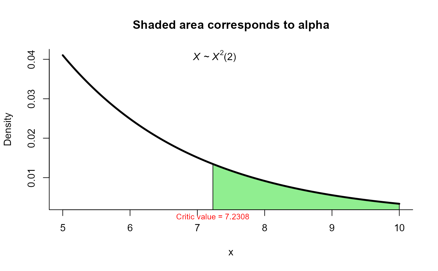
res2 <- two_mean_vector_test(xbar1 = xbar1, s1 = s1, n1 = n1,
xbar2 = xbar2, s2 = s2, n2 = n2,
method = 'james', alpha=0.05)
res2
#>
#> James test for two mean vectors
#>
#> data: this test uses summarized data
#> T2 = 9.4455, critic_value = 7.2308, df = 2
#> alternative hypothesis: mu1 is not equal to mu2
#>
#> sample estimates:
#> Sample 1 Sample 2
#> xbar_1 9.82 13.05
#> xbar_2 15.06 22.57
#>
plot(res2, from=5, to=10, shade.col="lightgreen")
# Example 3.7 from Seber (1984) page 116.
# using the James first order test (1954).
n1 <- 16
xbar1 <- c(9.82, 15.06)
s1 <- matrix(c(120, -16.3,
-16.3, 17.8), ncol = 2)
n2 <- 11
xbar2 <- c(13.05, 22.57)
s2 <- matrix(c(81.8, 32.1,
32.1, 53.8), ncol = 2)
res2 <- two_mean_vector_test(xbar1 = xbar1, s1 = s1, n1 = n1,
xbar2 = xbar2, s2 = s2, n2 = n2,
method = 'james', alpha=0.05)
res2
#>
#> James test for two mean vectors
#>
#> data: this test uses summarized data
#> T2 = 9.4455, critic_value = 7.2308, df = 2
#> alternative hypothesis: mu1 is not equal to mu2
#>
#> sample estimates:
#> Sample 1 Sample 2
#> xbar_1 9.82 13.05
#> xbar_2 15.06 22.57
#>
plot(res2, from=5, to=10, shade.col="lightgreen")
 # Example from page 141 from Yao (1965),
# using Yao's test
n1 <- 16
xbar1 <- c(9.82, 15.06)
s1 <- matrix(c(120, -16.3,
-16.3, 17.8), ncol = 2)
n2 <- 11
xbar2 <- c(13.05, 22.57)
s2 <- matrix(c(81.8, 32.1,
32.1, 53.8), ncol = 2)
res3 <- two_mean_vector_test(xbar1 = xbar1, s1 = s1, n1 = n1,
xbar2 = xbar2, s2 = s2, n2 = n2,
method = 'yao')
res3
#>
#> Yao test for two mean vectors
#>
#> data: this test uses summarized data
#> T2 = 9.4455, F = 4.3855, df1 = 2.000, df2 = 13.001, p-value = 0.03503
#> alternative hypothesis: mu1 is not equal to mu2
#>
#> sample estimates:
#> Sample 1 Sample 2
#> xbar_1 9.82 13.05
#> xbar_2 15.06 22.57
#>
plot(res3, from=2, to=6, shade.col="pink")
# Example from page 141 from Yao (1965),
# using Yao's test
n1 <- 16
xbar1 <- c(9.82, 15.06)
s1 <- matrix(c(120, -16.3,
-16.3, 17.8), ncol = 2)
n2 <- 11
xbar2 <- c(13.05, 22.57)
s2 <- matrix(c(81.8, 32.1,
32.1, 53.8), ncol = 2)
res3 <- two_mean_vector_test(xbar1 = xbar1, s1 = s1, n1 = n1,
xbar2 = xbar2, s2 = s2, n2 = n2,
method = 'yao')
res3
#>
#> Yao test for two mean vectors
#>
#> data: this test uses summarized data
#> T2 = 9.4455, F = 4.3855, df1 = 2.000, df2 = 13.001, p-value = 0.03503
#> alternative hypothesis: mu1 is not equal to mu2
#>
#> sample estimates:
#> Sample 1 Sample 2
#> xbar_1 9.82 13.05
#> xbar_2 15.06 22.57
#>
plot(res3, from=2, to=6, shade.col="pink")
 # Example for Johansen's test using the data from
# Example from page 141 from Yao (1965)
res4 <- two_mean_vector_test(xbar1 = xbar1, s1 = s1, n1 = n1,
xbar2 = xbar2, s2 = s2, n2 = n2,
method = 'johansen')
res4
#>
#> Johansen test for two mean vectors
#>
#> data: this test uses summarized data
#> T2 = 9.4455, F = 4.5476, df1 = 2.000, df2 = 16.309, p-value = 0.02587
#> alternative hypothesis: mu1 is not equal to mu2
#>
#> sample estimates:
#> Sample 1 Sample 2
#> xbar_1 9.82 13.05
#> xbar_2 15.06 22.57
#>
plot(res4, from=2, to=6, shade.col="aquamarine1")
# Example for Johansen's test using the data from
# Example from page 141 from Yao (1965)
res4 <- two_mean_vector_test(xbar1 = xbar1, s1 = s1, n1 = n1,
xbar2 = xbar2, s2 = s2, n2 = n2,
method = 'johansen')
res4
#>
#> Johansen test for two mean vectors
#>
#> data: this test uses summarized data
#> T2 = 9.4455, F = 4.5476, df1 = 2.000, df2 = 16.309, p-value = 0.02587
#> alternative hypothesis: mu1 is not equal to mu2
#>
#> sample estimates:
#> Sample 1 Sample 2
#> xbar_1 9.82 13.05
#> xbar_2 15.06 22.57
#>
plot(res4, from=2, to=6, shade.col="aquamarine1")
 # Example 4.1 from Nel and Van de Merwe (1986) page 3729
# Test H0: mu1 = mu2 versus H1: mu1 != mu2
n1 <- 45
xbar1 <- c(204.4, 556.6)
s1 <- matrix(c(13825.3, 23823.4,
23823.4, 73107.4), ncol=2)
n2 <- 55
xbar2 <- c(130.0, 355.0)
s2 <- matrix(c(8632.0, 19616.7,
19616.7, 55964.5), ncol=2)
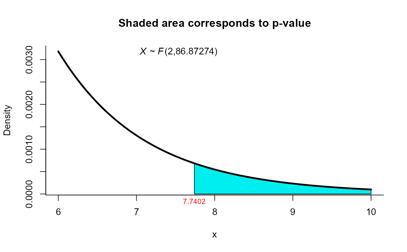
res5 <- two_mean_vector_test(xbar1 = xbar1, s1 = s1, n1 = n1,
xbar2 = xbar2, s2 = s2, n2 = n2,
method = 'nvm')
res5
#>
#> Nel and Van der Merwe test for two mean vectors
#>
#> data: this test uses summarized data
#> T2 = 15.6585, F = 7.7402, df1 = 2.000, df2 = 86.873, p-value =
#> 0.0008064
#> alternative hypothesis: mu1 is not equal to mu2
#>
#> sample estimates:
#> Sample 1 Sample 2
#> xbar_1 204.4 130
#> xbar_2 556.6 355
#>
plot(res5, from=6, to=10, shade.col='cyan2')
# Example 4.1 from Nel and Van de Merwe (1986) page 3729
# Test H0: mu1 = mu2 versus H1: mu1 != mu2
n1 <- 45
xbar1 <- c(204.4, 556.6)
s1 <- matrix(c(13825.3, 23823.4,
23823.4, 73107.4), ncol=2)
n2 <- 55
xbar2 <- c(130.0, 355.0)
s2 <- matrix(c(8632.0, 19616.7,
19616.7, 55964.5), ncol=2)
res5 <- two_mean_vector_test(xbar1 = xbar1, s1 = s1, n1 = n1,
xbar2 = xbar2, s2 = s2, n2 = n2,
method = 'nvm')
res5
#>
#> Nel and Van der Merwe test for two mean vectors
#>
#> data: this test uses summarized data
#> T2 = 15.6585, F = 7.7402, df1 = 2.000, df2 = 86.873, p-value =
#> 0.0008064
#> alternative hypothesis: mu1 is not equal to mu2
#>
#> sample estimates:
#> Sample 1 Sample 2
#> xbar_1 204.4 130
#> xbar_2 556.6 355
#>
plot(res5, from=6, to=10, shade.col='cyan2')
 # using mnvm method for same data
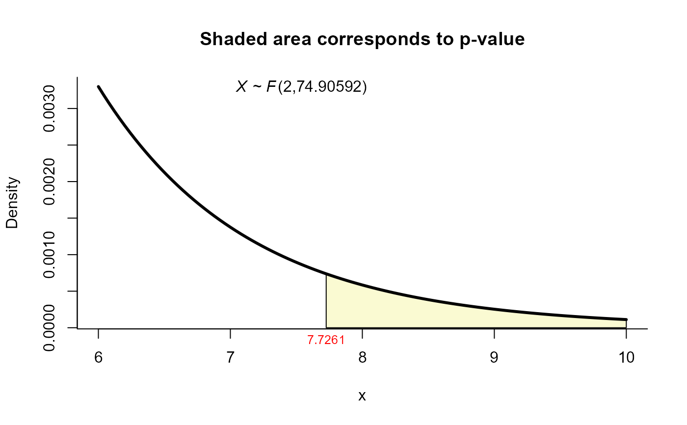
res6 <- two_mean_vector_test(xbar1 = xbar1, s1 = s1, n1 = n1,
xbar2 = xbar2, s2 = s2, n2 = n2,
method = 'mnvm')
res6
#>
#> Modified Nel and Van der Merwe test for two mean vectors
#>
#> data: this test uses summarized data
#> T2 = 15.6585, F = 7.7261, df1 = 2.000, df2 = 74.906, p-value = 0.00089
#> alternative hypothesis: mu1 is not equal to mu2
#>
#> sample estimates:
#> Sample 1 Sample 2
#> xbar_1 204.4 130
#> xbar_2 556.6 355
#>
plot(res6, from=6, to=10, shade.col='lightgoldenrodyellow')
# using mnvm method for same data
res6 <- two_mean_vector_test(xbar1 = xbar1, s1 = s1, n1 = n1,
xbar2 = xbar2, s2 = s2, n2 = n2,
method = 'mnvm')
res6
#>
#> Modified Nel and Van der Merwe test for two mean vectors
#>
#> data: this test uses summarized data
#> T2 = 15.6585, F = 7.7261, df1 = 2.000, df2 = 74.906, p-value = 0.00089
#> alternative hypothesis: mu1 is not equal to mu2
#>
#> sample estimates:
#> Sample 1 Sample 2
#> xbar_1 204.4 130
#> xbar_2 556.6 355
#>
plot(res6, from=6, to=10, shade.col='lightgoldenrodyellow')
 # using gamage method for same data
res7 <- two_mean_vector_test(xbar1 = xbar1, s1 = s1, n1 = n1,
xbar2 = xbar2, s2 = s2, n2 = n2,
method = 'gamage')
res7
#>
#> Gamage test for two mean vectors
#>
#> data: this test uses summarized data
#> T2 = 15.659, p-value = 5e-04
#> alternative hypothesis: mu1 is not equal to mu2
#>
#> sample estimates:
#> Sample 1 Sample 2
#> xbar_1 204.4 130
#> xbar_2 556.6 355
#>
plot(res7, from=0, to=20, shade.col='mediumpurple4')
text(x=10, y=0.30, "The curve corresponds to an empirical density",
col='orange')
# using gamage method for same data
res7 <- two_mean_vector_test(xbar1 = xbar1, s1 = s1, n1 = n1,
xbar2 = xbar2, s2 = s2, n2 = n2,
method = 'gamage')
res7
#>
#> Gamage test for two mean vectors
#>
#> data: this test uses summarized data
#> T2 = 15.659, p-value = 5e-04
#> alternative hypothesis: mu1 is not equal to mu2
#>
#> sample estimates:
#> Sample 1 Sample 2
#> xbar_1 204.4 130
#> xbar_2 556.6 355
#>
plot(res7, from=0, to=20, shade.col='mediumpurple4')
text(x=10, y=0.30, "The curve corresponds to an empirical density",
col='orange')
 # using Yanagihara and Yuan method for same data
res8 <- two_mean_vector_test(xbar1 = xbar1, s1 = s1, n1 = n1,
xbar2 = xbar2, s2 = s2, n2 = n2,
method = 'yy')
res8
#>
#> Yanagihara and Yuan test for two mean vectors
#>
#> data: this test uses summarized data
#> T2 = 15.6585, F = 7.7272, df1 = 2.000, df2 = 74.309, p-value =
#> 0.0008937
#> alternative hypothesis: mu1 is not equal to mu2
#>
#> sample estimates:
#> Sample 1 Sample 2
#> xbar_1 204.4 130
#> xbar_2 556.6 355
#>
plot(res8, from=6, to=10, shade.col='gold2')
# using Yanagihara and Yuan method for same data
res8 <- two_mean_vector_test(xbar1 = xbar1, s1 = s1, n1 = n1,
xbar2 = xbar2, s2 = s2, n2 = n2,
method = 'yy')
res8
#>
#> Yanagihara and Yuan test for two mean vectors
#>
#> data: this test uses summarized data
#> T2 = 15.6585, F = 7.7272, df1 = 2.000, df2 = 74.309, p-value =
#> 0.0008937
#> alternative hypothesis: mu1 is not equal to mu2
#>
#> sample estimates:
#> Sample 1 Sample 2
#> xbar_1 204.4 130
#> xbar_2 556.6 355
#>
plot(res8, from=6, to=10, shade.col='gold2')
 # using Bartlett Correction method for same data
res9 <- two_mean_vector_test(xbar1 = xbar1, s1 = s1, n1 = n1,
xbar2 = xbar2, s2 = s2, n2 = n2,
method = 'byy')
res9
#>
#> Bartlett Correction test for two mean vectors
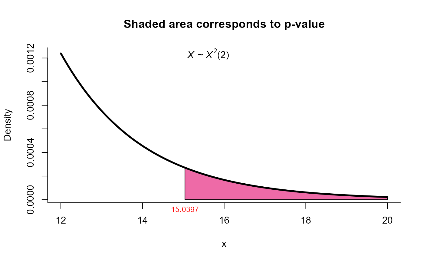
#>
#> data: this test uses summarized data
#> T2 = 15.659, X-squared = 15.040, df = 2, p-value = 0.0005422
#> alternative hypothesis: mu1 is not equal to mu2
#>
#> sample estimates:
#> Sample 1 Sample 2
#> xbar_1 204.4 130
#> xbar_2 556.6 355
#>
plot(res9, from=12, to=20, shade.col='hotpink2')
# using Bartlett Correction method for same data
res9 <- two_mean_vector_test(xbar1 = xbar1, s1 = s1, n1 = n1,
xbar2 = xbar2, s2 = s2, n2 = n2,
method = 'byy')
res9
#>
#> Bartlett Correction test for two mean vectors
#>
#> data: this test uses summarized data
#> T2 = 15.659, X-squared = 15.040, df = 2, p-value = 0.0005422
#> alternative hypothesis: mu1 is not equal to mu2
#>
#> sample estimates:
#> Sample 1 Sample 2
#> xbar_1 204.4 130
#> xbar_2 556.6 355
#>
plot(res9, from=12, to=20, shade.col='hotpink2')
 # using modified Bartlett Correction method for same data
res10 <- two_mean_vector_test(xbar1 = xbar1, s1 = s1, n1 = n1,
xbar2 = xbar2, s2 = s2, n2 = n2,
method = 'mbyy')
res10
#>
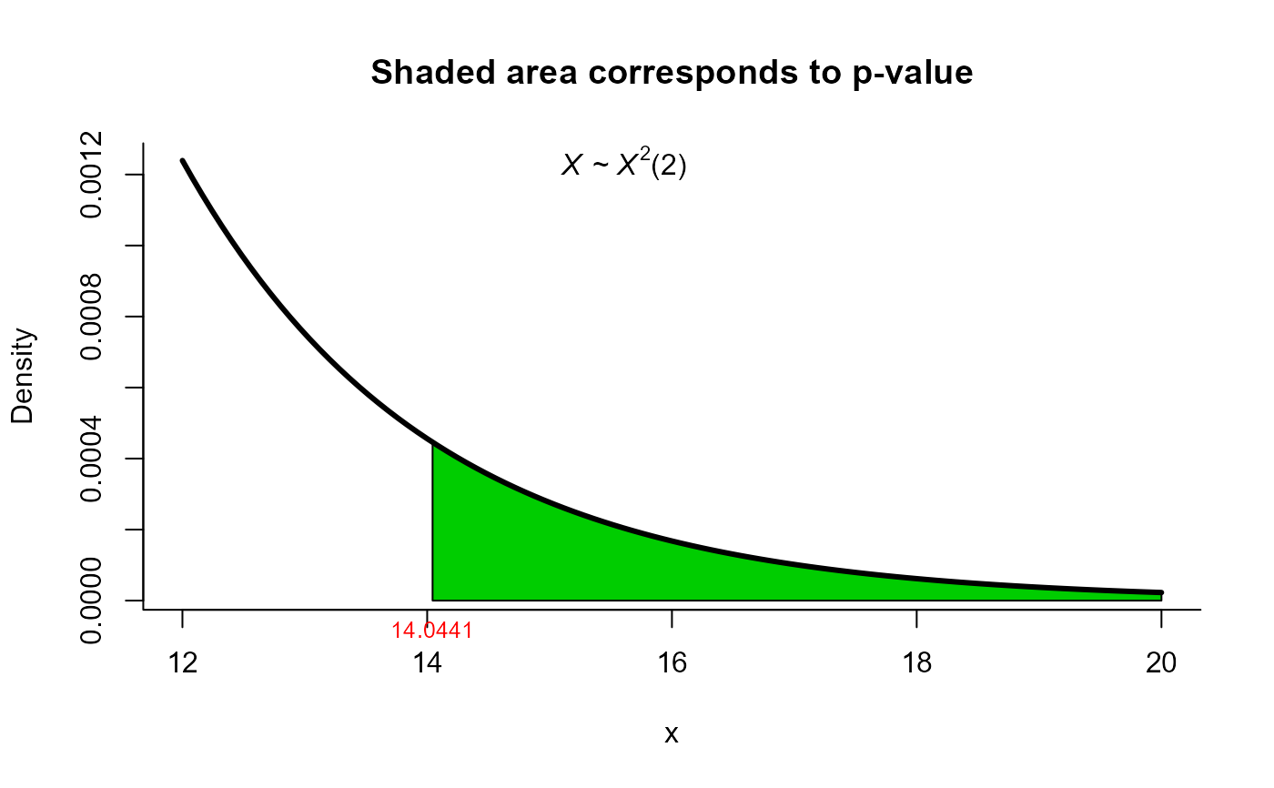
#> Modified Bartlett Correction test for two mean vectors
#>
#> data: this test uses summarized data
#> T2 = 15.659, X-squared = 14.044, df = 2, p-value = 0.000892
#> alternative hypothesis: mu1 is not equal to mu2
#>
#> sample estimates:
#> Sample 1 Sample 2
#> xbar_1 204.4 130
#> xbar_2 556.6 355
#>
plot(res10, from=12, to=20, shade.col='green3')
# using modified Bartlett Correction method for same data
res10 <- two_mean_vector_test(xbar1 = xbar1, s1 = s1, n1 = n1,
xbar2 = xbar2, s2 = s2, n2 = n2,
method = 'mbyy')
res10
#>
#> Modified Bartlett Correction test for two mean vectors
#>
#> data: this test uses summarized data
#> T2 = 15.659, X-squared = 14.044, df = 2, p-value = 0.000892
#> alternative hypothesis: mu1 is not equal to mu2
#>
#> sample estimates:
#> Sample 1 Sample 2
#> xbar_1 204.4 130
#> xbar_2 556.6 355
#>
plot(res10, from=12, to=20, shade.col='green3')
 # using Second Order Procedure (Kawasaki and Seo (2015)) method for same data
res11 <- two_mean_vector_test(xbar1 = xbar1, s1 = s1, n1 = n1,
xbar2 = xbar2, s2 = s2, n2 = n2,
method = 'ks1')
res11
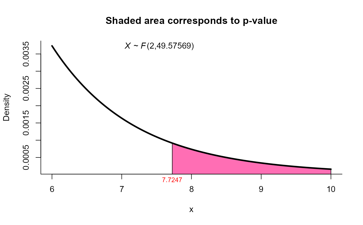
#>
#> Kawasaki and Seo (Second order) test for two mean vectors
#>
#> data: this test uses summarized data
#> T2 = 15.6585, F = 7.7247, df1 = 2.000, df2 = 49.576, p-value = 0.001201
#> alternative hypothesis: mu1 is not equal to mu2
#>
#> sample estimates:
#> Sample 1 Sample 2
#> xbar_1 204.4 130
#> xbar_2 556.6 355
#>
plot(res11, from=6, to=10, shade.col='hotpink1')
# using Second Order Procedure (Kawasaki and Seo (2015)) method for same data
res11 <- two_mean_vector_test(xbar1 = xbar1, s1 = s1, n1 = n1,
xbar2 = xbar2, s2 = s2, n2 = n2,
method = 'ks1')
res11
#>
#> Kawasaki and Seo (Second order) test for two mean vectors
#>
#> data: this test uses summarized data
#> T2 = 15.6585, F = 7.7247, df1 = 2.000, df2 = 49.576, p-value = 0.001201
#> alternative hypothesis: mu1 is not equal to mu2
#>
#> sample estimates:
#> Sample 1 Sample 2
#> xbar_1 204.4 130
#> xbar_2 556.6 355
#>
plot(res11, from=6, to=10, shade.col='hotpink1')
 # using Bias Correction Procedure (Kawasaki and Seo (2015)) method for same data
res12 <- two_mean_vector_test(xbar1 = xbar1, s1 = s1, n1 = n1,
xbar2 = xbar2, s2 = s2, n2 = n2,
method = 'ks2')
res12
#>
#> Kawasaki and Seo (Bias Correction) test for two mean vectors
#>
#> data: this test uses summarized data
#> T2 = 15.659, F = 7.714, df1 = 2.000, df2 = 47.075, p-value = 0.001266
#> alternative hypothesis: mu1 is not equal to mu2
#>
#> sample estimates:
#> Sample 1 Sample 2
#> xbar_1 204.4 130
#> xbar_2 556.6 355
#>
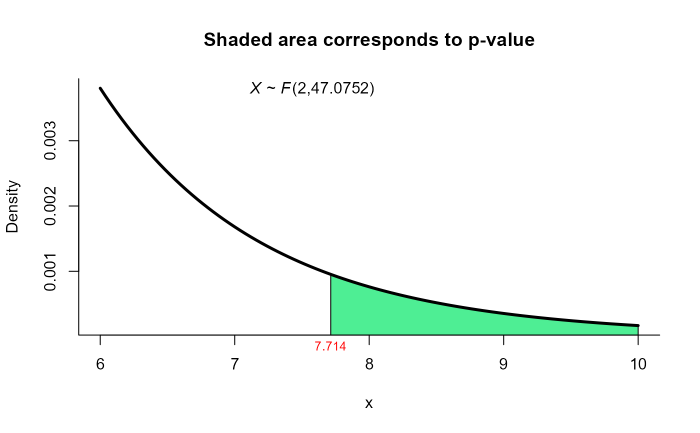
plot(res12, from=6, to=10, shade.col='seagreen2')
# using Bias Correction Procedure (Kawasaki and Seo (2015)) method for same data
res12 <- two_mean_vector_test(xbar1 = xbar1, s1 = s1, n1 = n1,
xbar2 = xbar2, s2 = s2, n2 = n2,
method = 'ks2')
res12
#>
#> Kawasaki and Seo (Bias Correction) test for two mean vectors
#>
#> data: this test uses summarized data
#> T2 = 15.659, F = 7.714, df1 = 2.000, df2 = 47.075, p-value = 0.001266
#> alternative hypothesis: mu1 is not equal to mu2
#>
#> sample estimates:
#> Sample 1 Sample 2
#> xbar_1 204.4 130
#> xbar_2 556.6 355
#>
plot(res12, from=6, to=10, shade.col='seagreen2')