Tests for homogeneity of covariances matrices — mult_var_matrices

The function implements the test for \(H_0: \Sigma_1 = \Sigma_2 = ... = \Sigma_g\) versus \(H_1\) at least one \(\Sigma_i\) is different.

mult_var_matrices_test(S, N, method = "box")

Arguments

S: a list with the sample covariance matrices.
N: a list with the sample sizes.
method: a character string specifying the method, "box" (default), please see the details section for other methods.

Value

A list with class "htest" containing the following components:

statistic: the value of the statistic.
parameter: the degrees of freedom for the test.
p.value: the p-value for the test.
estimate: the estimated mean vectors.
method: a character string indicating the type of test performed.

Details

the "method" must be one of "box" (default), "modified_LRT", "wald_schott".

To know in detail all tests implemented here the reader can visit the vignette https://fhernanb.github.io/stests/articles/Tests_Sigmas.html

References

Schott, J. R. (2001). Some tests for the equality of covariance matrices. Journal of statistical planning and inference, 94(1), 25-36.

Schott, J. R. (2007). A test for the equality of covariance matrices when the dimension is large relative to the sample sizes. Computational Statistics & Data Analysis, 51(12), 6535-6542.

Mardia, K. V., Kent, J. T., & Bibby, J. M. (1979). Multivariate analysis.

Author

Freddy Hernandez.

Examples

# Example 5.2.3 from Diaz and Morales (2015) page 200
S1 <- matrix(c(12.65, -16.45,
               -16.45, 73.04), ncol=2, nrow=2)
S2 <- matrix(c(11.44, -27.77,
               -27.77, 100.64), ncol=2, nrow=2)
S3 <- matrix(c(14.46, -31.26,
               -31.26, 101.03), ncol=2, nrow=2)
N1 <- 26
N2 <- 23
N3 <- 25
S <- list(S1, S2, S3)
N <- list(N1, N2, N3)

res <- mult_var_matrices_test(S=S, N=N, method="box")
res
#> 
#> 	Box test for homogeneity of covariances
#> 
#> data:  this test uses summarized data
#> phi = 6.6472, df = 6, p-value = 0.3547
#> alternative hypothesis: at least one covariance matrix is different 
#> 
#> sample estimates:
#> [1] "Due to the high value of m, matrices S1, ..., S3 are not displayed."
#> 
plot(res, shade.col="tomato")


# Example 5.3.4 from Mardia (1979) page 141
S1 <- matrix(c(132.99, 75.85, 35.82,
               75.85, 47.96, 20.75,
               35.82, 20.75, 10.79), ncol=3, nrow=3)
S2 <- matrix(c(432.58, 259.87, 161.67,
               259.87, 164.57, 98.99,
               161.67, 98.99, 63.87), ncol=3, nrow=3)
N1 <- 24
N2 <- 24
S <- list(S1, S2)
N <- list(N1, N2)

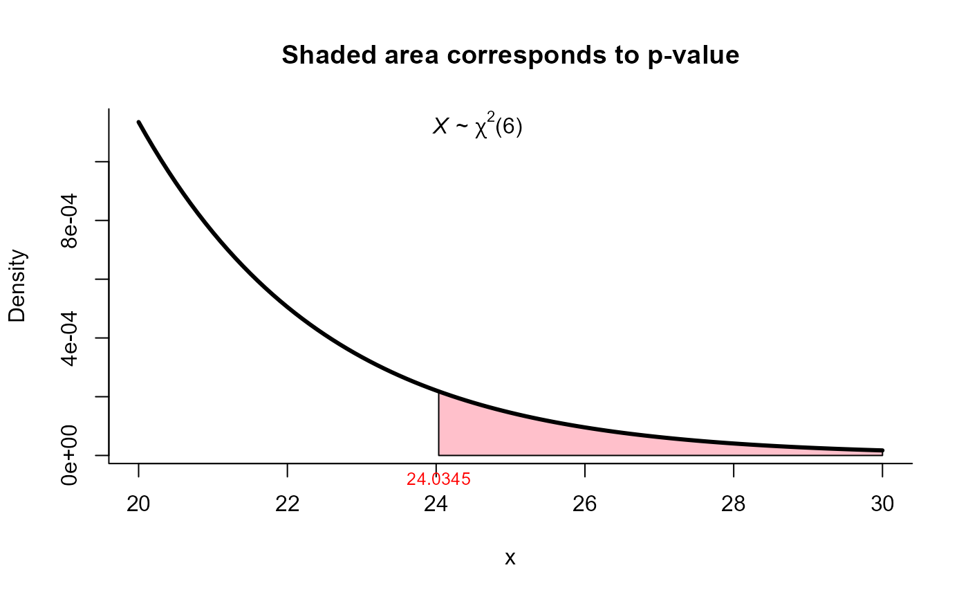
res <- mult_var_matrices_test(S=S, N=N, method="modified_LRT")
res
#> 
#> 	Modified likelihood ratio (or Bartlett's) test for homogeneity of
#> 	covariances
#> 
#> data:  this test uses summarized data
#> M = 25.862, df = 6, p-value = 0.0002362
#> alternative hypothesis: at least one covariance matrix is different 
#> 
#> sample estimates:
#> [1] "Due to the high value of m, matrices S1, ..., S2 are not displayed."
#> 
plot(res, from=20, to=30, shade.col="pink")


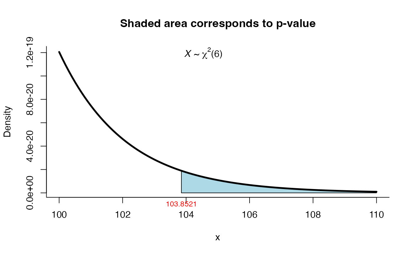
res <- mult_var_matrices_test(S=S, N=N, method="wald_schott")
res
#> 
#> 	Wald-Schott test for homogeneity of covariances
#> 
#> data:  this test uses summarized data
#> W = 103.85, df = 6, p-value < 2.2e-16
#> alternative hypothesis: the covariance matrices are different 
#> 
#> sample estimates:
#> [1] "Due to the high value of m, matrices S1, ..., S2 are not displayed."
#> 
plot(res, from=100, to=110, shade.col="lightblue")