The Discrete Poisson XLindley

These functions define the density, distribution function, quantile function and random generation for the Discrete Poisson XLindley distribution with parameter \(\mu\).

dPOISXL(x, mu = 0.3, log = FALSE)

pPOISXL(q, mu = 0.3, lower.tail = TRUE, log.p = FALSE)

qPOISXL(p, mu = 0.3, lower.tail = TRUE, log.p = FALSE)

rPOISXL(n, mu = 0.3)

Arguments

x, q: vector of (non-negative integer) quantiles.
mu: vector of the mu parameter.
log, log.p: logical; if TRUE, probabilities p are given as log(p).
lower.tail: logical; if TRUE (default), probabilities are \(P[X <= x]\), otherwise, P[X > x].
p: vector of probabilities.
n: number of random values to return

Value

dPOISXL gives the density, pPOISXL gives the distribution function, qPOISXL gives the quantile function, rPOISXL

generates random deviates.

Details

The Discrete Poisson XLindley distribution with parameters \(\mu\) has a support 0, 1, 2, ... and mass function given by

\(f(x | \mu) = \frac{\mu^2(x+\mu^2+3(1+\mu))}{(1+\mu)^{4+x}}\); with \(\mu>0\).

Note: in this implementation we changed the original parameters \(\alpha\) for \(\mu\), we did it to implement this distribution within gamlss framework.

References

Ahsan-ul-Haq M, Al-Bossly A, El-Morshedy M, Eliwa MS, others (2022). “Poisson XLindley distribution for count data: statistical and reliability properties with estimation techniques and inference.” Computational Intelligence and Neuroscience, 2022.

Author

Mariana Blandon Mejia, mblandonm@unal.edu.co

Examples

# Example 1
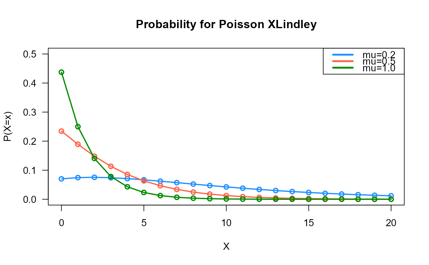
# Plotting the mass function for different parameter values

x_max <- 20
probs1 <- dPOISXL(x=0:x_max, mu=0.2)
probs2 <- dPOISXL(x=0:x_max, mu=0.5)
probs3 <- dPOISXL(x=0:x_max, mu=1.0)

# To plot the first k values
plot(x=0:x_max, y=probs1, type="o", lwd=2, col="dodgerblue", las=1,
     ylab="P(X=x)", xlab="X", main="Probability for Poisson XLindley",
     ylim=c(0, 0.50))
points(x=0:x_max, y=probs2, type="o", lwd=2, col="tomato")
points(x=0:x_max, y=probs3, type="o", lwd=2, col="green4")
legend("topright", col=c("dodgerblue", "tomato", "green4"), lwd=3,
       legend=c("mu=0.2", "mu=0.5", "mu=1.0"))


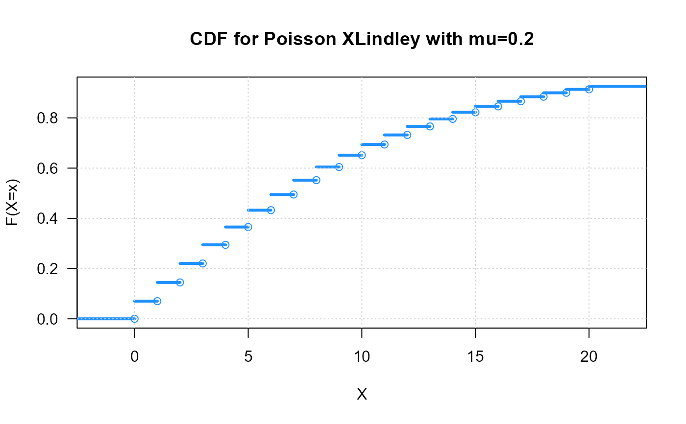
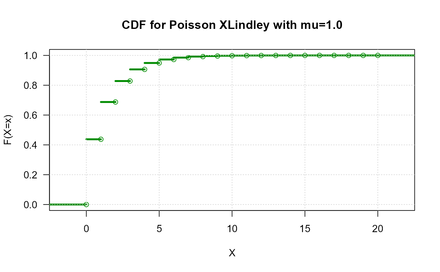
# Example 2
# Checking if the cumulative curves converge to 1

x_max <- 20

plot_discrete_cdf(x=0:x_max,
                  fx=dPOISXL(x=0:x_max, mu=0.2), col="dodgerblue",
                  main="CDF for Poisson XLindley with mu=0.2")


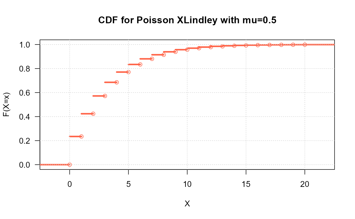
plot_discrete_cdf(x=0:x_max,
                  fx=dPOISXL(x=0:x_max, mu=0.5), col="tomato",
                  main="CDF for Poisson XLindley with mu=0.5")


plot_discrete_cdf(x=0:x_max,
                  fx=dPOISXL(x=0:x_max, mu=1.0), col="green4",
                  main="CDF for Poisson XLindley with mu=1.0")


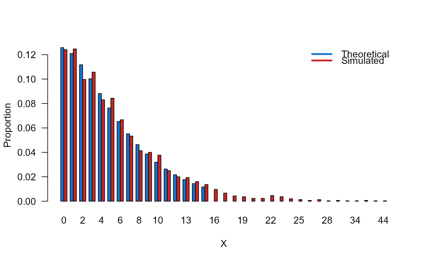
# Example 3
# Comparing the random generator output with
# the theoretical probabilities

x_max <- 15
probs1 <- dPOISXL(x=0:x_max, mu=0.3)
names(probs1) <- 0:x_max

x <- rPOISXL(n=3000, mu=0.3)
probs2 <- prop.table(table(x))

cn <- union(names(probs1), names(probs2))
height <- rbind(probs1[cn], probs2[cn])
nombres <- cn
mp <- barplot(height, beside = TRUE, names.arg = nombres,
              col=c("dodgerblue3","firebrick3"), las=1,
              xlab="X", ylab="Proportion")
legend("topright",
       legend=c("Theoretical", "Simulated"),
       bty="n", lwd=3,
       col=c("dodgerblue3","firebrick3"), lty=1)


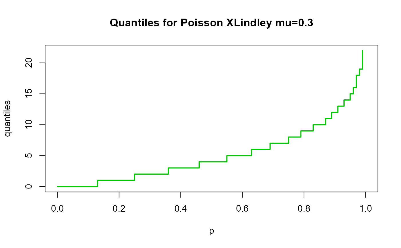
# Example 4
# Checking the quantile function

mu <- 0.3
p <- seq(from=0, to=1, by = 0.01)
qxx <- qPOISXL(p, mu, lower.tail = TRUE, log.p = FALSE)
plot(p, qxx, type="s", lwd=2, col="green3", ylab="quantiles",
     main="Quantiles for Poisson XLindley mu=0.3")

References

Ahsan-ul-Haq, M., Al-Bossly, A., El-Morshedy, M., & Eliwa, M. S. (2022). Poisson XLindley distribution for count data: statistical and reliability properties with estimation techniques and inference. Computational Intelligence and neuroscience, 2022(1), 6503670.