These functions define the density, distribution function, quantile function and random generation for the hyper-Poisson in the second parameterization with parameters \(\mu\) (as mean) and \(\sigma\) as the dispersion parameter.
dHYPERPO2(x, mu = 1, sigma = 1, log = FALSE)

pHYPERPO2(q, mu = 1, sigma = 1, lower.tail = TRUE, log.p = FALSE)

rHYPERPO2(n, mu = 1, sigma = 1)

qHYPERPO2(p, mu = 1, sigma = 1, lower.tail = TRUE, log.p = FALSE)
Arguments
- x, q
vector of (non-negative integer) quantiles.
- mu
vector of positive values of this parameter.
- sigma
vector of positive values of this parameter.
- log, log.p
logical; if TRUE, probabilities p are given as log(p).
- lower.tail
logical; if TRUE (default), probabilities are \(P[X <= x]\), otherwise, \(P[X > x]\).
- n
number of random values to return
- p
vector of probabilities.
Value
dHYPERPO2 gives the density, pHYPERPO2 gives the distribution
function, qHYPERPO2 gives the quantile function, rHYPERPO2
generates random deviates.
Details
The hyper-Poisson distribution with parameters \(\mu\) and \(\sigma\) has a support 0, 1, 2, ...
Note: in this implementation the parameter \(\mu\) is the mean of the distribution and \(\sigma\) corresponds to the dispersion parameter. If you fit a model with this parameterization, the time will increase because an internal procedure to convert \(\mu\) to \(\lambda\) parameter.
References
Sáez-Castillo, A. J., & Conde-Sánchez, A. (2013). A hyper-Poisson regression model for overdispersed and underdispersed count data. Computational Statistics & Data Analysis, 61, 148-157.
Examples
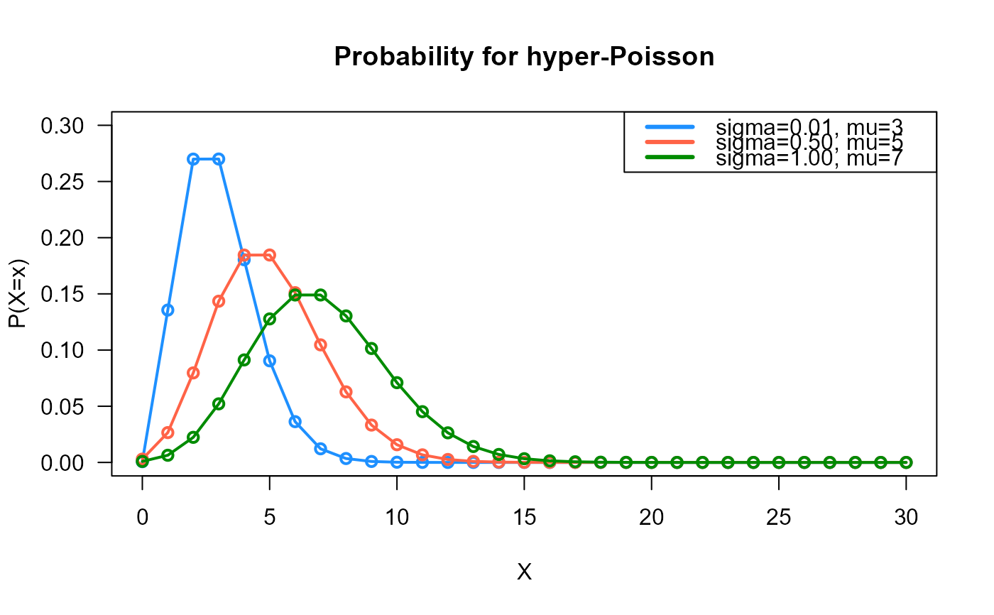
# Example 1
# Plotting the mass function for different parameter values
x_max <- 30
probs1 <- dHYPERPO2(x=0:x_max, sigma=0.01, mu=3)
probs2 <- dHYPERPO2(x=0:x_max, sigma=0.50, mu=5)
probs3 <- dHYPERPO2(x=0:x_max, sigma=1.00, mu=7)
# To plot the first k values
plot(x=0:x_max, y=probs1, type="o", lwd=2, col="dodgerblue", las=1,
ylab="P(X=x)", xlab="X", main="Probability for hyper-Poisson",
ylim=c(0, 0.30))
points(x=0:x_max, y=probs2, type="o", lwd=2, col="tomato")
points(x=0:x_max, y=probs3, type="o", lwd=2, col="green4")
legend("topright", col=c("dodgerblue", "tomato", "green4"), lwd=3,
legend=c("sigma=0.01, mu=3",
"sigma=0.50, mu=5",
"sigma=1.00, mu=7"))
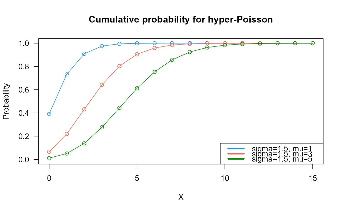
 # Example 2
# Checking if the cumulative curves converge to 1
x_max <- 15
cumulative_probs1 <- pHYPERPO2(q=0:x_max, mu=1, sigma=1.5)
cumulative_probs2 <- pHYPERPO2(q=0:x_max, mu=3, sigma=1.5)
cumulative_probs3 <- pHYPERPO2(q=0:x_max, mu=5, sigma=1.5)
plot(x=0:x_max, y=cumulative_probs1, col="dodgerblue",
type="o", las=1, ylim=c(0, 1),
main="Cumulative probability for hyper-Poisson",
xlab="X", ylab="Probability")
points(x=0:x_max, y=cumulative_probs2, type="o", col="tomato")
points(x=0:x_max, y=cumulative_probs3, type="o", col="green4")
legend("bottomright", col=c("dodgerblue", "tomato", "green4"), lwd=3,
legend=c("sigma=1.5, mu=1",
"sigma=1.5, mu=3",
"sigma=1.5, mu=5"))
# Example 2
# Checking if the cumulative curves converge to 1
x_max <- 15
cumulative_probs1 <- pHYPERPO2(q=0:x_max, mu=1, sigma=1.5)
cumulative_probs2 <- pHYPERPO2(q=0:x_max, mu=3, sigma=1.5)
cumulative_probs3 <- pHYPERPO2(q=0:x_max, mu=5, sigma=1.5)
plot(x=0:x_max, y=cumulative_probs1, col="dodgerblue",
type="o", las=1, ylim=c(0, 1),
main="Cumulative probability for hyper-Poisson",
xlab="X", ylab="Probability")
points(x=0:x_max, y=cumulative_probs2, type="o", col="tomato")
points(x=0:x_max, y=cumulative_probs3, type="o", col="green4")
legend("bottomright", col=c("dodgerblue", "tomato", "green4"), lwd=3,
legend=c("sigma=1.5, mu=1",
"sigma=1.5, mu=3",
"sigma=1.5, mu=5"))
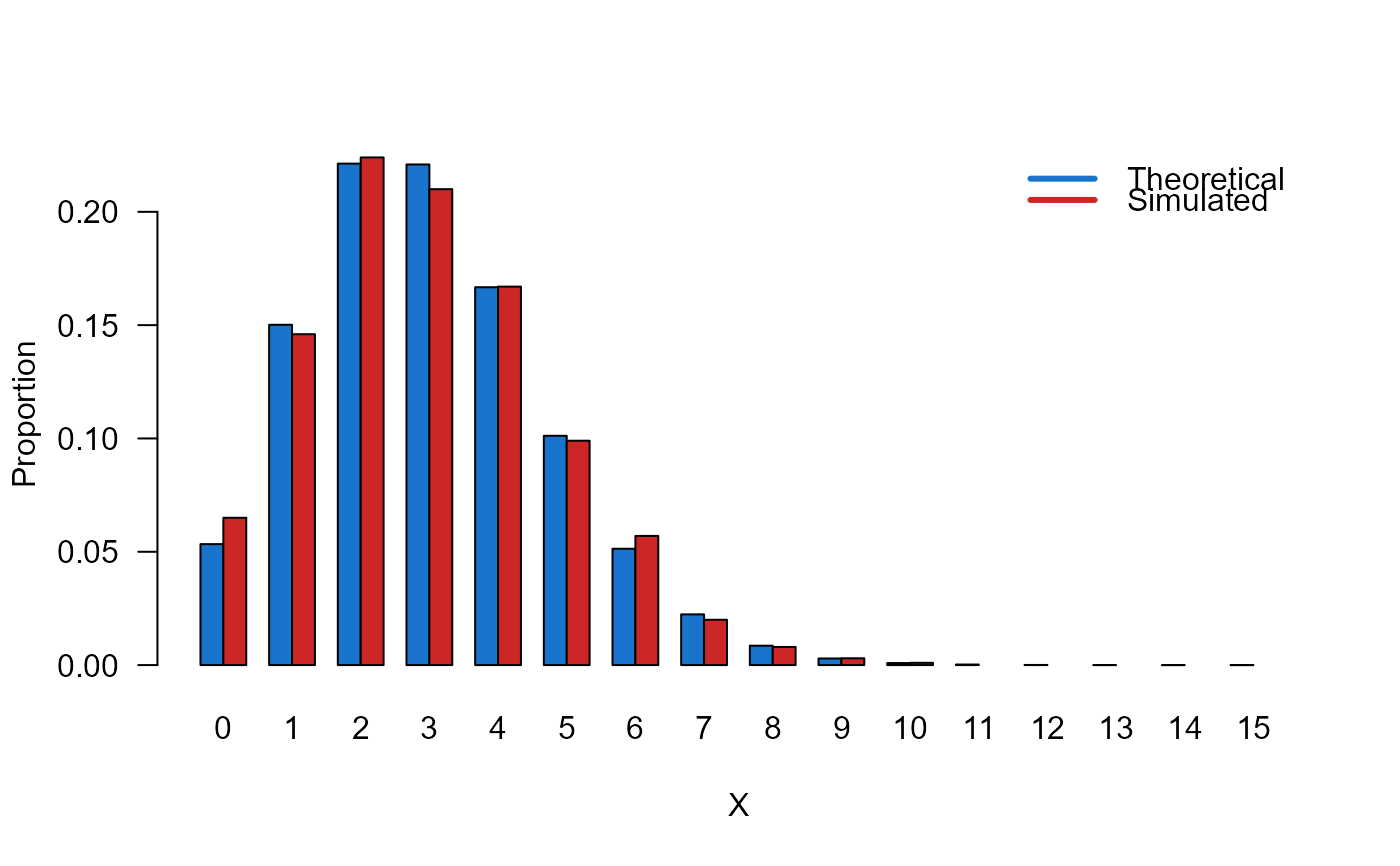
 # Example 3
# Comparing the random generator output with
# the theoretical probabilities
x_max <- 15
probs1 <- dHYPERPO2(x=0:x_max, mu=3, sigma=1.1)
names(probs1) <- 0:x_max
x <- rHYPERPO2(n=1000, mu=3, sigma=1.1)
probs2 <- prop.table(table(x))
cn <- union(names(probs1), names(probs2))
height <- rbind(probs1[cn], probs2[cn])
nombres <- cn
mp <- barplot(height, beside = TRUE, names.arg = nombres,
col=c('dodgerblue3','firebrick3'), las=1,
xlab='X', ylab='Proportion')
legend('topright',
legend=c('Theoretical', 'Simulated'),
bty='n', lwd=3,
col=c('dodgerblue3','firebrick3'), lty=1)
# Example 3
# Comparing the random generator output with
# the theoretical probabilities
x_max <- 15
probs1 <- dHYPERPO2(x=0:x_max, mu=3, sigma=1.1)
names(probs1) <- 0:x_max
x <- rHYPERPO2(n=1000, mu=3, sigma=1.1)
probs2 <- prop.table(table(x))
cn <- union(names(probs1), names(probs2))
height <- rbind(probs1[cn], probs2[cn])
nombres <- cn
mp <- barplot(height, beside = TRUE, names.arg = nombres,
col=c('dodgerblue3','firebrick3'), las=1,
xlab='X', ylab='Proportion')
legend('topright',
legend=c('Theoretical', 'Simulated'),
bty='n', lwd=3,
col=c('dodgerblue3','firebrick3'), lty=1)
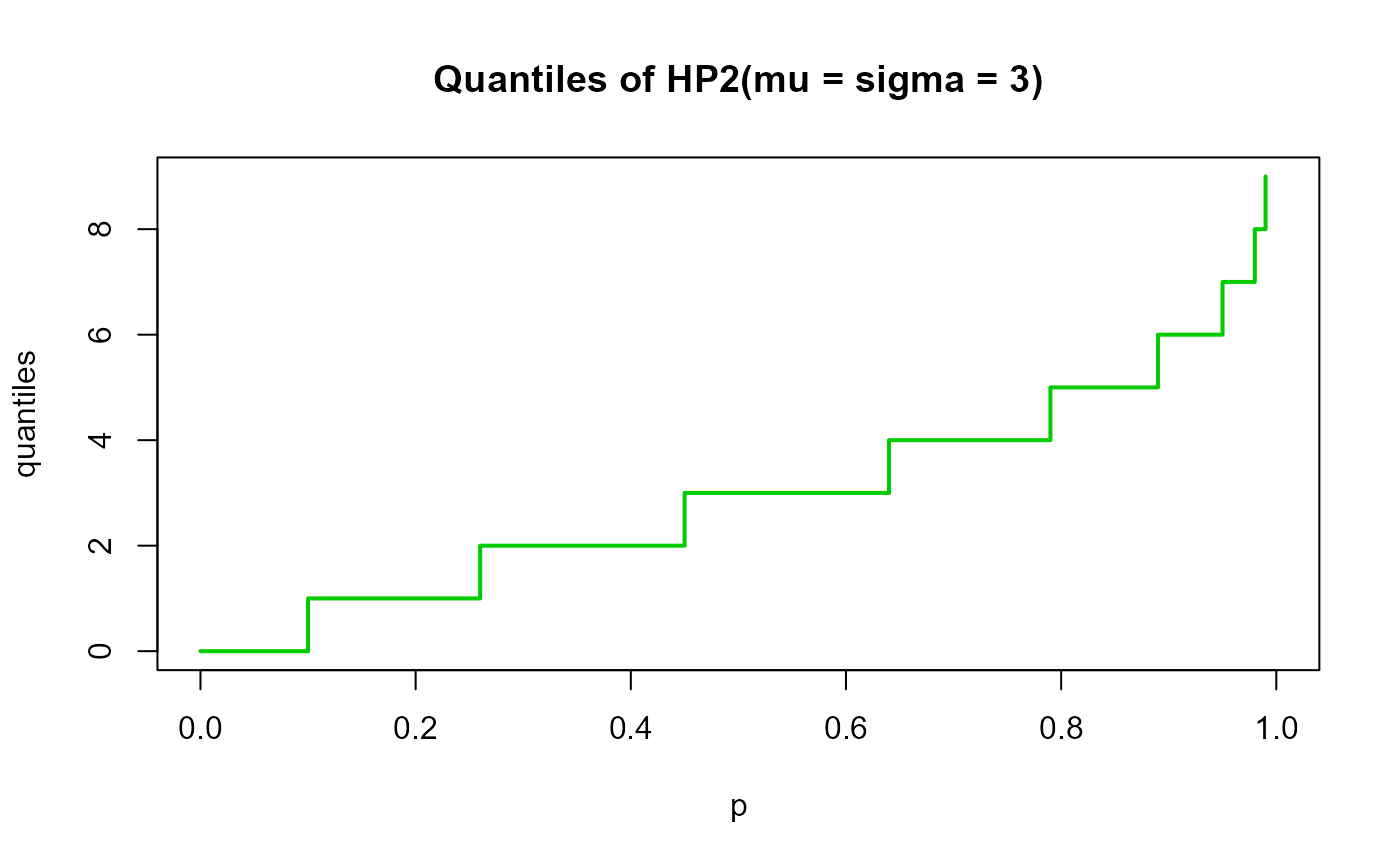
 # Example 4
# Checking the quantile function
mu <- 3
sigma <-3
p <- seq(from=0, to=1, by=0.01)
qxx <- qHYPERPO2(p=p, mu=mu, sigma=sigma, lower.tail=TRUE, log.p=FALSE)
plot(p, qxx, type="s", lwd=2, col="green3", ylab="quantiles",
main="Quantiles of HP2(mu = sigma = 3)")
# Example 4
# Checking the quantile function
mu <- 3
sigma <-3
p <- seq(from=0, to=1, by=0.01)
qxx <- qHYPERPO2(p=p, mu=mu, sigma=sigma, lower.tail=TRUE, log.p=FALSE)
plot(p, qxx, type="s", lwd=2, col="green3", ylab="quantiles",
main="Quantiles of HP2(mu = sigma = 3)")