These functions define the density, distribution function, quantile function and random generation for the Discrete Marshall–Olkin Length Biased Exponential DMOLBE distribution with parameters \(\mu\) and \(\sigma\).
dDMOLBE(x, mu = 1, sigma = 1, log = FALSE)

pDMOLBE(q, mu = 1, sigma = 1, lower.tail = TRUE, log.p = FALSE)

rDMOLBE(n, mu = 1, sigma = 1)

qDMOLBE(p, mu = 1, sigma = 1, lower.tail = TRUE, log.p = FALSE)
Arguments
- x, q
vector of (non-negative integer) quantiles.
- mu
vector of the mu parameter.
- sigma
vector of the sigma parameter.
- log, log.p
logical; if TRUE, probabilities p are given as log(p).
- lower.tail
logical; if TRUE (default), probabilities are \(P[X <= x]\), otherwise, \(P[X > x]\).
- n
number of random values to return.
- p
vector of probabilities.
Value
dDMOLBE gives the density, pDMOLBE gives the distribution
function, qDMOLBE gives the quantile function, rDMOLBE
generates random deviates.
Details
The DMOLBE distribution with parameters \(\mu\) and \(\sigma\) has a support 0, 1, 2, ... and mass function given by
\(f(x | \mu, \sigma) = \frac{\sigma ((1+x/\mu)\exp(-x/\mu)-(1+(x+1)/\mu)\exp(-(x+1)/\mu))}{(1-(1-\sigma)(1+x/\mu)\exp(-x/\mu)) ((1-(1-\sigma)(1+(x+1)/\mu)\exp(-(x+1)/\mu))}\)
with \(\mu > 0\) and \(\sigma > 0\)
References
Aljohani, H. M., Ahsan-ul-Haq, M., Zafar, J., Almetwally, E. M., Alghamdi, A. S., Hussam, E., & Muse, A. H. (2023). Analysis of Covid-19 data using discrete Marshall–Olkinin length biased exponential: Bayesian and frequentist approach. Scientific Reports, 13(1), 12243.
See also
Examples
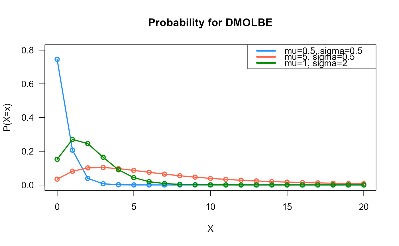
# Example 1
# Plotting the mass function for different parameter values
x_max <- 20
probs1 <- dDMOLBE(x=0:x_max, mu=0.5, sigma=0.5)
probs2 <- dDMOLBE(x=0:x_max, mu=5, sigma=0.5)
probs3 <- dDMOLBE(x=0:x_max, mu=1, sigma=2)
# To plot the first k values
plot(x=0:x_max, y=probs1, type="o", lwd=2, col="dodgerblue", las=1,
ylab="P(X=x)", xlab="X", main="Probability for DMOLBE",
ylim=c(0, 0.80))
points(x=0:x_max, y=probs2, type="o", lwd=2, col="tomato")
points(x=0:x_max, y=probs3, type="o", lwd=2, col="green4")
legend("topright", col=c("dodgerblue", "tomato", "green4"), lwd=3,
legend=c("mu=0.5, sigma=0.5",
"mu=5, sigma=0.5",
"mu=1, sigma=2"))
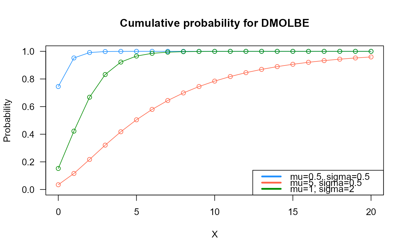
 # Example 2
# Checking if the cumulative curves converge to 1
x_max <- 20
cumulative_probs1 <- pDMOLBE(q=0:x_max, mu=0.5, sigma=0.5)
cumulative_probs2 <- pDMOLBE(q=0:x_max, mu=5, sigma=0.5)
cumulative_probs3 <- pDMOLBE(q=0:x_max, mu=1, sigma=2)
plot(x=0:x_max, y=cumulative_probs1, col="dodgerblue",
type="o", las=1, ylim=c(0, 1),
main="Cumulative probability for DMOLBE",
xlab="X", ylab="Probability")
points(x=0:x_max, y=cumulative_probs2, type="o", col="tomato")
points(x=0:x_max, y=cumulative_probs3, type="o", col="green4")
legend("bottomright", col=c("dodgerblue", "tomato", "green4"), lwd=3,
legend=c("mu=0.5, sigma=0.5",
"mu=5, sigma=0.5",
"mu=1, sigma=2"))
# Example 2
# Checking if the cumulative curves converge to 1
x_max <- 20
cumulative_probs1 <- pDMOLBE(q=0:x_max, mu=0.5, sigma=0.5)
cumulative_probs2 <- pDMOLBE(q=0:x_max, mu=5, sigma=0.5)
cumulative_probs3 <- pDMOLBE(q=0:x_max, mu=1, sigma=2)
plot(x=0:x_max, y=cumulative_probs1, col="dodgerblue",
type="o", las=1, ylim=c(0, 1),
main="Cumulative probability for DMOLBE",
xlab="X", ylab="Probability")
points(x=0:x_max, y=cumulative_probs2, type="o", col="tomato")
points(x=0:x_max, y=cumulative_probs3, type="o", col="green4")
legend("bottomright", col=c("dodgerblue", "tomato", "green4"), lwd=3,
legend=c("mu=0.5, sigma=0.5",
"mu=5, sigma=0.5",
"mu=1, sigma=2"))
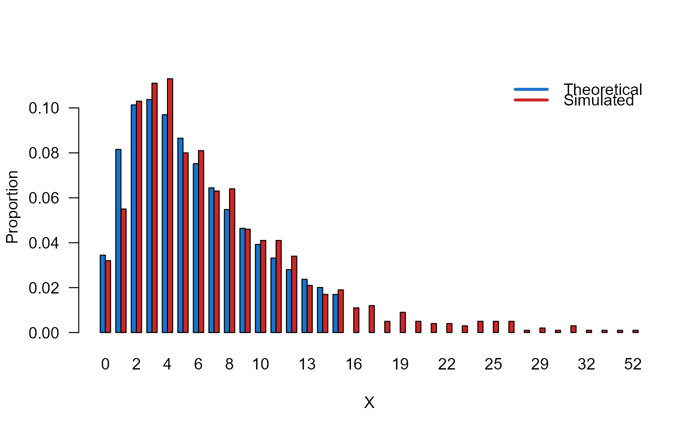
 # Example 3
# Comparing the random generator output with
# the theoretical probabilities
x_max <- 50
probs1 <- dDMOLBE(x=0:x_max, mu=5, sigma=0.5)
names(probs1) <- 0:x_max
x <- rDMOLBE(n=1000, mu=5, sigma=0.5)
probs2 <- prop.table(table(x))
cn <- union(names(probs1), names(probs2))
height <- rbind(probs1[cn], probs2[cn])
mp <- barplot(height, beside = TRUE, names.arg = cn,
col=c("dodgerblue3","firebrick3"), las=1,
xlab="X", ylab="Proportion")
legend("topright",
legend=c("Theoretical", "Simulated"),
bty="n", lwd=3,
col=c("dodgerblue3","firebrick3"), lty=1)
# Example 3
# Comparing the random generator output with
# the theoretical probabilities
x_max <- 50
probs1 <- dDMOLBE(x=0:x_max, mu=5, sigma=0.5)
names(probs1) <- 0:x_max
x <- rDMOLBE(n=1000, mu=5, sigma=0.5)
probs2 <- prop.table(table(x))
cn <- union(names(probs1), names(probs2))
height <- rbind(probs1[cn], probs2[cn])
mp <- barplot(height, beside = TRUE, names.arg = cn,
col=c("dodgerblue3","firebrick3"), las=1,
xlab="X", ylab="Proportion")
legend("topright",
legend=c("Theoretical", "Simulated"),
bty="n", lwd=3,
col=c("dodgerblue3","firebrick3"), lty=1)
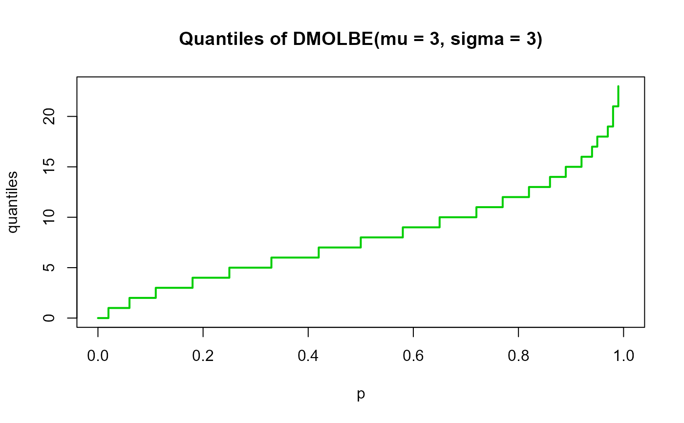
 # Example 4
# Checking the quantile function
mu <- 3
sigma <-3
p <- seq(from=0, to=1, by=0.01)
qxx <- qDMOLBE(p=p, mu=mu, sigma=sigma, lower.tail=TRUE, log.p=FALSE)
plot(p, qxx, type="s", lwd=2, col="green3", ylab="quantiles",
main="Quantiles of DMOLBE(mu = 3, sigma = 3)")
# Example 4
# Checking the quantile function
mu <- 3
sigma <-3
p <- seq(from=0, to=1, by=0.01)
qxx <- qDMOLBE(p=p, mu=mu, sigma=sigma, lower.tail=TRUE, log.p=FALSE)
plot(p, qxx, type="s", lwd=2, col="green3", ylab="quantiles",
main="Quantiles of DMOLBE(mu = 3, sigma = 3)")