The Kumaraswamy Inverse Weibull distribution

Density, distribution function, quantile function, random generation and hazard function for the Kumaraswamy Inverse Weibull distribution with parameters mu, sigma and nu.

Usage

dKumIW(x, mu, sigma, nu, log = FALSE)

pKumIW(q, mu, sigma, nu, lower.tail = TRUE, log.p = FALSE)

qKumIW(p, mu, sigma, nu, lower.tail = TRUE, log.p = FALSE)

rKumIW(n, mu, sigma, nu)

hKumIW(x, mu, sigma, nu)

Arguments

x, q

vector of quantiles.

mu

parameter.

sigma

parameter.

nu

parameter.

log, log.p

logical; if TRUE, probabilities p are given as log(p).

lower.tail

logical; if TRUE (default), probabilities are P[X <= x], otherwise, P[X > x].

p

vector of probabilities.

n

number of observations.

Value

dKumIW gives the density, pKumIW gives the distribution function, qKumIW gives the quantile function, rKumIW generates random deviates and hKumIW gives the hazard function.

Details

The Kumaraswamy Inverse Weibull Distribution with parameters mu, sigma and nu has density given by

\(f(x)= \mu \sigma \nu x^{-\mu - 1} \exp{- \sigma x^{-\mu}} (1 - \exp{- \sigma x^{-\mu}})^{\nu - 1},\)

for \(x > 0\), \(\mu > 0\), \(\sigma > 0\) and \(\nu > 0\).

References

Almalki, S. J., & Nadarajah, S. (2014). Modifications of the Weibull distribution: A review. Reliability Engineering & System Safety, 124, 32-55.

Shahbaz, M. Q., Shahbaz, S., & Butt, N. S. (2012). The Kumaraswamy Inverse Weibull Distribution. Pakistan journal of statistics and operation research, 479-489.

See also

KumIW

Author

Johan David Marin Benjumea, johand.marin@udea.edu.co

Examples

old_par <- par(mfrow = c(1, 1)) # save previous graphical parameters

## The probability density function 
par(mfrow = c(1, 1))
curve(dKumIW(x, mu = 1.5, sigma=  1.5, nu = 1), from = 0, to = 8.5, 
      col = "red", las = 1, ylab = "f(x)")


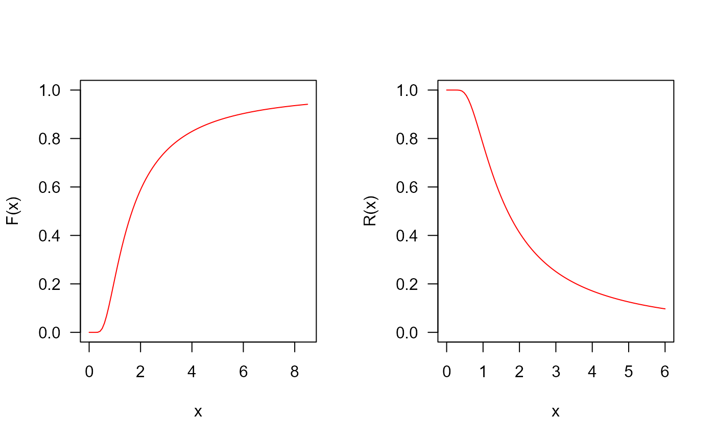
## The cumulative distribution and the Reliability function
par(mfrow = c(1, 2))
curve(pKumIW(x, mu = 1.5, sigma=  1.5, nu = 1), from = 0, to = 8.5, 
      ylim = c(0, 1), col = "red", las = 1, ylab = "F(x)")
curve(pKumIW(x, mu = 1.5, sigma=  1.5, nu = 1, lower.tail = FALSE), 
      from = 0, to = 6, ylim = c(0, 1), col = "red", las = 1, ylab = "R(x)")


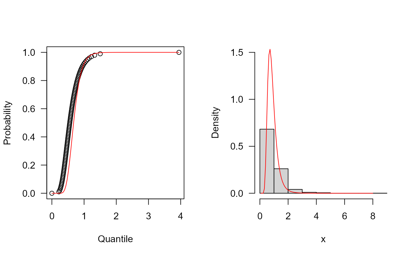
## The quantile function
p <- seq(from = 0, to = 0.99999, length.out = 100)
plot(x = qKumIW(p=p, mu = 1.5, sigma=  1.5, nu = 10), y = p, 
     xlab = "Quantile", las = 1, ylab = "Probability")
curve(pKumIW(x, mu = 1.5, sigma=  1.5, nu = 10), from = 0, add = TRUE, 
      col = "red")

## The random function
hist(rKumIW(1000, mu = 1.5, sigma=  1.5, nu = 5), freq = FALSE, xlab = "x", 
     las = 1, ylim = c(0, 1.5), main = "")
curve(dKumIW(x, mu = 1.5, sigma=  1.5, nu = 5), from = 0, to =8, add = TRUE, 
      col = "red")


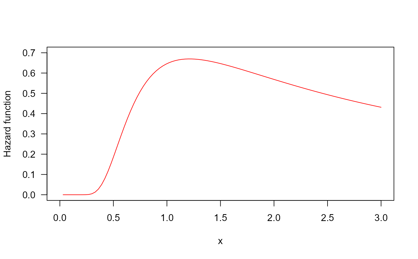
## The Hazard function
par(mfrow=c(1,1))
curve(hKumIW(x, mu = 1.5, sigma=  1.5, nu = 1), from = 0, to = 3, 
      ylim = c(0, 0.7), col = "red", ylab = "Hazard function", las = 1)


par(old_par) # restore previous graphical parameters