This function obtains the probability for the Bivariate Poisson distribution under the parameterization of Lakshminarayana et. al (1993).
dBP_Laksh(x, l1, l2, alpha, log = FALSE)

rBP_Laksh(n, l1, l2, alpha, max_val_x1 = NULL, max_val_x2 = NULL)
Arguments
- x
vector or matrix of quantiles. When
xis a matrix, each row is taken to be a quantile and columns correspond to the number of dimensionsp.- l1
mean for the marginal \(X_1\) variable with Poisson distribution.
- l2
mean for the marginal \(X_2\) variable with Poisson distribution.
- alpha
third parameter.
- log
logical; if
TRUE, densities d are given as log(d).- n
number of random observations.
- max_val_x1
maximum value for \(X_1\) that is expected, by default it is 100.
- max_val_x2
maximum value for \(X_2\) that is expected, by default it is 100.
Value
Returns the density for a given data x.
References
Lakshminarayana, J., Pandit, S. N., & Srinivasa Rao, K. (1999). On a bivariate Poisson distribution. Communications in Statistics-Theory and Methods, 28(2), 267-276.
Examples
# Example 1 ---------------------------------------------------------------
# Probability for single values of X1 and X2
dBP_Laksh(c(0, 0), l1=3, l2=4, alpha=1)
#> [1] 0.001625049
dBP_Laksh(c(1, 0), l1=3, l2=4, alpha=1)
#> [1] 0.003283848
dBP_Laksh(c(0, 1), l1=3, l2=4, alpha=1)
#> [1] 0.004540631
# Probability for a matrix the values of X1 and X2
x <- matrix(c(0, 0,
1, 0,
0, 1), ncol=2, byrow=TRUE)
x
#> [,1] [,2]
#> [1,] 0 0
#> [2,] 1 0
#> [3,] 0 1
dBP_Laksh(x=x, l1=3, l2=4, alpha=1)
#> [1] 0.001625049 0.003283848 0.004540631
# Checking if the probabilities sum 1
val_x1 <- val_x2 <- 0:50
space <- expand.grid(val_x1, val_x2)
space <- as.matrix(space)
l1 <- 3
l2 <- 4
alpha <- -1.27
probs <- dBP_Laksh(x=space, l1=l1, l2=l2, alpha=alpha)
sum(probs)
#> [1] 1
# Example 2 ---------------------------------------------------------------
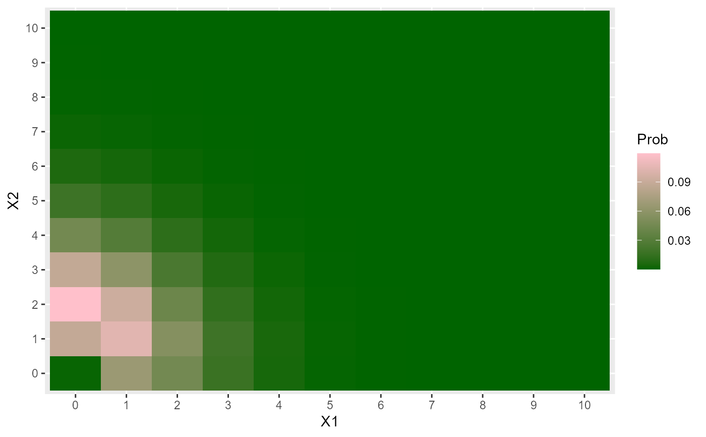
# Heat map for a BP_Laksh
l1 <- 1
l2 <- 2
correct_alpha_BP_Laksh(l1=l1, l2=l2)
#> $min_alpha
#> [1] -2.97445
#>
#> $max_alpha
#> [1] 2.97445
#>
alpha <- -2.9
X1 <- 0:10
X2 <- 0:10
data <- expand.grid(X1=X1, X2=X2)
data$Prob <- dBP_Laksh(x=data, l1=l1, l2=l2, alpha=alpha)
data$X1 <- factor(data$X1)
data$X2 <- factor(data$X2)
library(ggplot2)
ggplot(data, aes(X1, X2, fill=Prob)) +
geom_tile() +
scale_fill_gradient(low="darkgreen", high="pink")
 # Example 3 ---------------------------------------------------------------
# Generating random values and moment estimations
l1 <- 1
l2 <- 2
correct_alpha_BP_Laksh(l1=l1, l2=l2)
#> $min_alpha
#> [1] -2.97445
#>
#> $max_alpha
#> [1] 2.97445
#>
alpha <- -2.7
x <- rBP_Laksh(n=500, l1, l2, alpha)
moments_estim_BP_Laksh(x)
#> l1_hat l2_hat alpha_hat_cor
#> 0.9880 2.0460 -2.4809
# Example 4 ---------------------------------------------------------------
# Estimating the parameters using the loglik function
# Loglik function
llBP_Laksh <- function(param, x) {
l1 <- param[1] # param: is the parameter vector
l2 <- param[2]
alpha <- param[3]
sum(dBP_Laksh(x=x, l1=l1, l2=l2, alpha=alpha, log=TRUE))
}
# The known parameters
l1 <- 1
l2 <- 2
correct_alpha_BP_Laksh(l1=l1, l2=l2)
#> $min_alpha
#> [1] -2.97445
#>
#> $max_alpha
#> [1] 2.97445
#>
alpha <- -2.7
set.seed(12345)
x <- rBP_Laksh(n=500, l1=l1, l2=l2, alpha=alpha)
# To obtain reasonable values for alpha
theta <- as.numeric(moments_estim_BP_Laksh(x))
theta
#> [1] 1.1020 1.9640 -2.7606
# To create start parameters
min_alpha <- correct_alpha_BP_Laksh(l1=theta[1],
l2=theta[2])$min_alpha
max_alpha <- correct_alpha_BP_Laksh(l1=theta[1],
l2=theta[2])$max_alpha
start_param <- theta
names(start_param) <- c("l1_hat", "l2_hat", "alpha_hat")
start_param
#> l1_hat l2_hat alpha_hat
#> 1.1020 1.9640 -2.7606
# Estimating parameters
res1 <- optim(fn = llBP_Laksh,
par = start_param,
lower = c(0.001, 0.001, min_alpha),
upper = c( Inf, Inf, max_alpha),
method = "L-BFGS-B",
control = list(maxit=100000, fnscale=-1),
x=x)
res1
#> $par
#> l1_hat l2_hat alpha_hat
#> 1.101373 1.957413 -2.566542
#>
#> $value
#> [1] -1507.214
#>
#> $counts
#> function gradient
#> 11 11
#>
#> $convergence
#> [1] 0
#>
#> $message
#> [1] "CONVERGENCE: REL_REDUCTION_OF_F <= FACTR*EPSMCH"
#>
# Analizing example of Laksh (1999) ---------------------------------------
x <- rep(0:5, each=6)
y <- rep(0:5, times=6)
freq <- c(7, 41, 54, 40, 21, 9,
36, 79, 83, 59, 30, 13,
39, 70, 69, 47, 25, 10,
24, 41, 39, 26, 14, 6,
10, 18, 18, 11, 6, 2,
3, 6, 6, 4, 2, 1)
seed_plants <- NULL
for (i in 1:36) {
temp <- matrix(c(x[i], y[i]), ncol=2, nrow=freq[i], byrow=TRUE)
seed_plants <- rbind(seed_plants, temp)
}
head(seed_plants)
#> [,1] [,2]
#> [1,] 0 0
#> [2,] 0 0
#> [3,] 0 0
#> [4,] 0 0
#> [5,] 0 0
#> [6,] 0 0
# Exploring some statistics
colMeans(seed_plants)
#> [1] 1.692466 2.013416
var(seed_plants)
#> [,1] [,2]
#> [1,] 1.5540857 -0.1539278
#> [2,] -0.1539278 1.7343240
cor(seed_plants)
#> [,1] [,2]
#> [1,] 1.00000000 -0.09375929
#> [2,] -0.09375929 1.00000000
# Moment estimators
moments_estim_BP_Laksh(seed_plants)
#> l1_hat l2_hat alpha_hat_cor
#> 1.6925 2.0134 -1.3230
# Correct interval for alpha according to l1_hat and l2_hat
correct_alpha_BP_Laksh(l1=1.6925, l2=2.0134)
#> $min_alpha
#> [1] -2.114373
#>
#> $max_alpha
#> [1] 2.114373
#>
# Finding the log-likelihood estimators using
optim(fn = llBP_Laksh,
par = c(1.6925, 2.0134, -1.3230),
lower = c(0.0001, 0.0001, -2.114373),
upper = c(Inf, Inf, 2.114373),
method = "L-BFGS-B",
control = list(maxit=100000, fnscale=-1),
x=seed_plants)
#> $par
#> [1] 1.698306 2.016876 -1.383463
#>
#> $value
#> [1] -3142.296
#>
#> $counts
#> function gradient
#> 12 12
#>
#> $convergence
#> [1] 0
#>
#> $message
#> [1] "CONVERGENCE: REL_REDUCTION_OF_F <= FACTR*EPSMCH"
#>
# Example 3 ---------------------------------------------------------------
# Generating random values and moment estimations
l1 <- 1
l2 <- 2
correct_alpha_BP_Laksh(l1=l1, l2=l2)
#> $min_alpha
#> [1] -2.97445
#>
#> $max_alpha
#> [1] 2.97445
#>
alpha <- -2.7
x <- rBP_Laksh(n=500, l1, l2, alpha)
moments_estim_BP_Laksh(x)
#> l1_hat l2_hat alpha_hat_cor
#> 0.9880 2.0460 -2.4809
# Example 4 ---------------------------------------------------------------
# Estimating the parameters using the loglik function
# Loglik function
llBP_Laksh <- function(param, x) {
l1 <- param[1] # param: is the parameter vector
l2 <- param[2]
alpha <- param[3]
sum(dBP_Laksh(x=x, l1=l1, l2=l2, alpha=alpha, log=TRUE))
}
# The known parameters
l1 <- 1
l2 <- 2
correct_alpha_BP_Laksh(l1=l1, l2=l2)
#> $min_alpha
#> [1] -2.97445
#>
#> $max_alpha
#> [1] 2.97445
#>
alpha <- -2.7
set.seed(12345)
x <- rBP_Laksh(n=500, l1=l1, l2=l2, alpha=alpha)
# To obtain reasonable values for alpha
theta <- as.numeric(moments_estim_BP_Laksh(x))
theta
#> [1] 1.1020 1.9640 -2.7606
# To create start parameters
min_alpha <- correct_alpha_BP_Laksh(l1=theta[1],
l2=theta[2])$min_alpha
max_alpha <- correct_alpha_BP_Laksh(l1=theta[1],
l2=theta[2])$max_alpha
start_param <- theta
names(start_param) <- c("l1_hat", "l2_hat", "alpha_hat")
start_param
#> l1_hat l2_hat alpha_hat
#> 1.1020 1.9640 -2.7606
# Estimating parameters
res1 <- optim(fn = llBP_Laksh,
par = start_param,
lower = c(0.001, 0.001, min_alpha),
upper = c( Inf, Inf, max_alpha),
method = "L-BFGS-B",
control = list(maxit=100000, fnscale=-1),
x=x)
res1
#> $par
#> l1_hat l2_hat alpha_hat
#> 1.101373 1.957413 -2.566542
#>
#> $value
#> [1] -1507.214
#>
#> $counts
#> function gradient
#> 11 11
#>
#> $convergence
#> [1] 0
#>
#> $message
#> [1] "CONVERGENCE: REL_REDUCTION_OF_F <= FACTR*EPSMCH"
#>
# Analizing example of Laksh (1999) ---------------------------------------
x <- rep(0:5, each=6)
y <- rep(0:5, times=6)
freq <- c(7, 41, 54, 40, 21, 9,
36, 79, 83, 59, 30, 13,
39, 70, 69, 47, 25, 10,
24, 41, 39, 26, 14, 6,
10, 18, 18, 11, 6, 2,
3, 6, 6, 4, 2, 1)
seed_plants <- NULL
for (i in 1:36) {
temp <- matrix(c(x[i], y[i]), ncol=2, nrow=freq[i], byrow=TRUE)
seed_plants <- rbind(seed_plants, temp)
}
head(seed_plants)
#> [,1] [,2]
#> [1,] 0 0
#> [2,] 0 0
#> [3,] 0 0
#> [4,] 0 0
#> [5,] 0 0
#> [6,] 0 0
# Exploring some statistics
colMeans(seed_plants)
#> [1] 1.692466 2.013416
var(seed_plants)
#> [,1] [,2]
#> [1,] 1.5540857 -0.1539278
#> [2,] -0.1539278 1.7343240
cor(seed_plants)
#> [,1] [,2]
#> [1,] 1.00000000 -0.09375929
#> [2,] -0.09375929 1.00000000
# Moment estimators
moments_estim_BP_Laksh(seed_plants)
#> l1_hat l2_hat alpha_hat_cor
#> 1.6925 2.0134 -1.3230
# Correct interval for alpha according to l1_hat and l2_hat
correct_alpha_BP_Laksh(l1=1.6925, l2=2.0134)
#> $min_alpha
#> [1] -2.114373
#>
#> $max_alpha
#> [1] 2.114373
#>
# Finding the log-likelihood estimators using
optim(fn = llBP_Laksh,
par = c(1.6925, 2.0134, -1.3230),
lower = c(0.0001, 0.0001, -2.114373),
upper = c(Inf, Inf, 2.114373),
method = "L-BFGS-B",
control = list(maxit=100000, fnscale=-1),
x=seed_plants)
#> $par
#> [1] 1.698306 2.016876 -1.383463
#>
#> $value
#> [1] -3142.296
#>
#> $counts
#> function gradient
#> 12 12
#>
#> $convergence
#> [1] 0
#>
#> $message
#> [1] "CONVERGENCE: REL_REDUCTION_OF_F <= FACTR*EPSMCH"
#>