These functions define the density, distribution function, quantile function and random generation for the Poisson–transmuted record type exponential (PTRTE) distribution with parameters \(\mu\) and \(\sigma\).
This distribution was proposed by Erbayram and Akdogan (2025) as a new discrete distribution obtained from a mixed Poisson model, where the Poisson parameter follows a transmuted record type exponential distribution.
dPTRTE(x, mu, sigma, log = FALSE)

pPTRTE(q, mu, sigma, lower.tail = TRUE, log.p = FALSE)

qPTRTE(p, mu, sigma, lower.tail = TRUE, log.p = FALSE)

rPTRTE(n, mu, sigma)
Arguments
- x, q
vector of (non-negative integer) quantiles.
- mu
vector of the mu parameter.
- sigma
vector of the sigma parameter.
- log, log.p
logical; if TRUE, probabilities p are given as log(p).
- lower.tail
logical; if TRUE (default), probabilities are \(P[X <= x]\), otherwise, \(P[X > x]\).
- p
vector of probabilities.
- n
number of random values to return.
Value
dPTRTE gives the density,
pPTRTE gives the distribution function,
qPTRTE gives the quantile function,
rPTRTE generates random deviates.
Details
The Poisson–transmuted record type exponential distribution with parameters \(\mu\) and \(\sigma\) has support \(x = 0,1,2,\dots\) and probability mass function given by
$$f(x | \mu, \sigma) = \frac{\mu}{(1+\mu)^{x+1}} \left(\frac{\sigma \mu (1+x)}{1+\mu} - (\sigma-1) \right)$$
with \(\mu > 0\) and \(0 < \sigma < 1\).
References
Erbayram, T., & Akdogan, Y. (2025). A new discrete model generated from mixed Poisson transmuted record type exponential distribution. Ricerca di Matematica, 74, 1225–1247.
See also
Examples
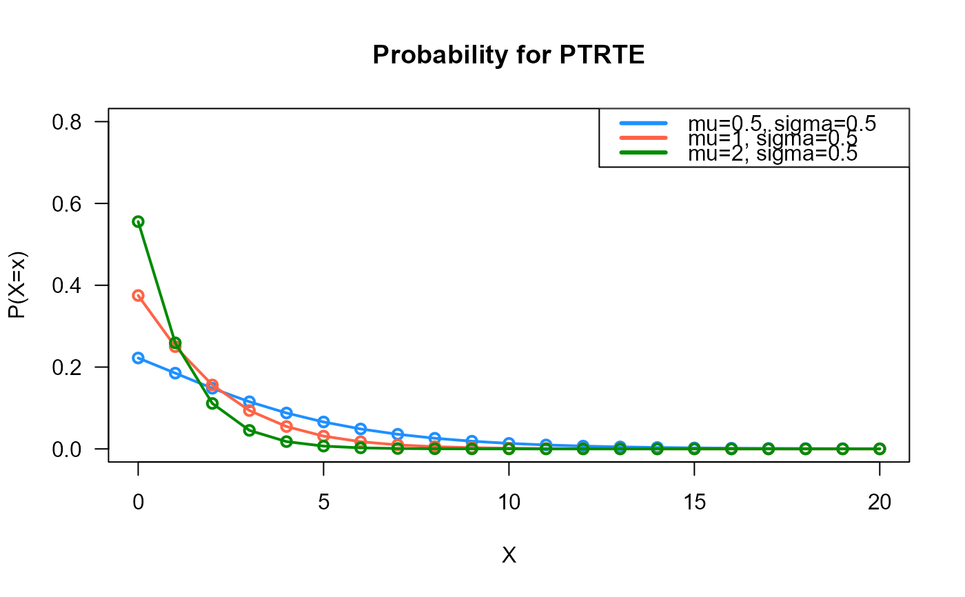
# Example 1
# Plotting the mass function for different parameter values
x_max <- 20
probs1 <- dPTRTE(x=0:x_max, mu=0.5, sigma=0.5)
probs2 <- dPTRTE(x=0:x_max, mu=1, sigma=0.5)
probs3 <- dPTRTE(x=0:x_max, mu=2, sigma=0.5)
# To plot the first k values
plot(x=0:x_max, y=probs1, type="o", lwd=2, col="dodgerblue", las=1,
ylab="P(X=x)", xlab="X", main="Probability for PTRTE",
ylim=c(0, 0.80))
points(x=0:x_max, y=probs2, type="o", lwd=2, col="tomato")
points(x=0:x_max, y=probs3, type="o", lwd=2, col="green4")
legend("topright", col=c("dodgerblue", "tomato", "green4"), lwd=3,
legend=c("mu=0.5, sigma=0.5",
"mu=1, sigma=0.5",
"mu=2, sigma=0.5"))
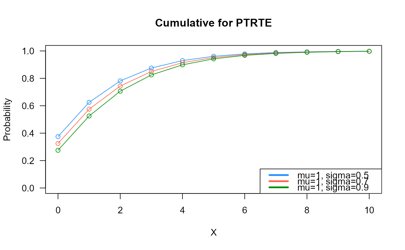
 # Example 2
# Checking if the cumulative curves converge to 1
x_max <- 10
cumulative_probs1 <- pPTRTE(q=0:x_max, mu=1, sigma=0.5)
cumulative_probs2 <- pPTRTE(q=0:x_max, mu=1, sigma=0.7)
cumulative_probs3 <- pPTRTE(q=0:x_max, mu=1, sigma=0.9)
plot(x=0:x_max, y=cumulative_probs1, col="dodgerblue",
type="o", las=1, ylim=c(0, 1),
main="Cumulative for PTRTE",
xlab="X", ylab="Probability")
points(x=0:x_max, y=cumulative_probs2, type="o", col="tomato")
points(x=0:x_max, y=cumulative_probs3, type="o", col="green4")
legend("bottomright", col=c("dodgerblue", "tomato", "green4"), lwd=3,
legend=c("mu=1, sigma=0.5",
"mu=1, sigma=0.7",
"mu=1, sigma=0.9"))
# Example 2
# Checking if the cumulative curves converge to 1
x_max <- 10
cumulative_probs1 <- pPTRTE(q=0:x_max, mu=1, sigma=0.5)
cumulative_probs2 <- pPTRTE(q=0:x_max, mu=1, sigma=0.7)
cumulative_probs3 <- pPTRTE(q=0:x_max, mu=1, sigma=0.9)
plot(x=0:x_max, y=cumulative_probs1, col="dodgerblue",
type="o", las=1, ylim=c(0, 1),
main="Cumulative for PTRTE",
xlab="X", ylab="Probability")
points(x=0:x_max, y=cumulative_probs2, type="o", col="tomato")
points(x=0:x_max, y=cumulative_probs3, type="o", col="green4")
legend("bottomright", col=c("dodgerblue", "tomato", "green4"), lwd=3,
legend=c("mu=1, sigma=0.5",
"mu=1, sigma=0.7",
"mu=1, sigma=0.9"))
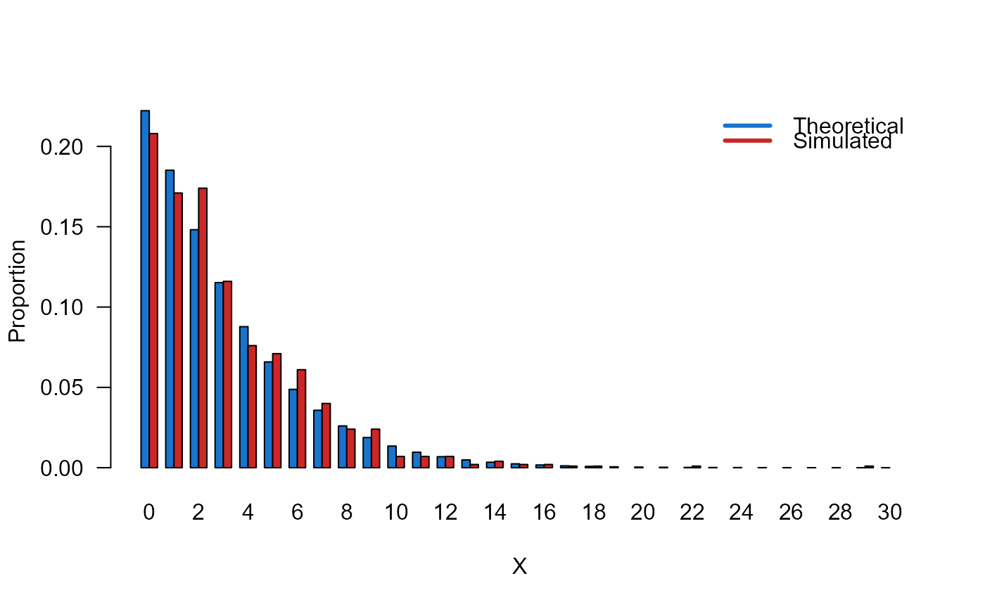
 # Example 3
# Comparing the random generator output with
# the theoretical probabilities
x_max <- 30
probs1 <- dPTRTE(x=0:x_max, mu=0.5, sigma=0.5)
names(probs1) <- 0:x_max
x <- rPTRTE(n=1000, mu=0.5, sigma=0.5)
probs2 <- prop.table(table(x))
cn <- union(names(probs1), names(probs2))
height <- rbind(probs1[cn], probs2[cn])
mp <- barplot(height, beside=TRUE, names.arg=cn,
col=c("dodgerblue3","firebrick3"), las=1,
xlab="X", ylab="Proportion")
legend("topright",
legend=c("Theoretical", "Simulated"),
bty="n", lwd=3,
col=c("dodgerblue3","firebrick3"), lty=1)
# Example 3
# Comparing the random generator output with
# the theoretical probabilities
x_max <- 30
probs1 <- dPTRTE(x=0:x_max, mu=0.5, sigma=0.5)
names(probs1) <- 0:x_max
x <- rPTRTE(n=1000, mu=0.5, sigma=0.5)
probs2 <- prop.table(table(x))
cn <- union(names(probs1), names(probs2))
height <- rbind(probs1[cn], probs2[cn])
mp <- barplot(height, beside=TRUE, names.arg=cn,
col=c("dodgerblue3","firebrick3"), las=1,
xlab="X", ylab="Proportion")
legend("topright",
legend=c("Theoretical", "Simulated"),
bty="n", lwd=3,
col=c("dodgerblue3","firebrick3"), lty=1)
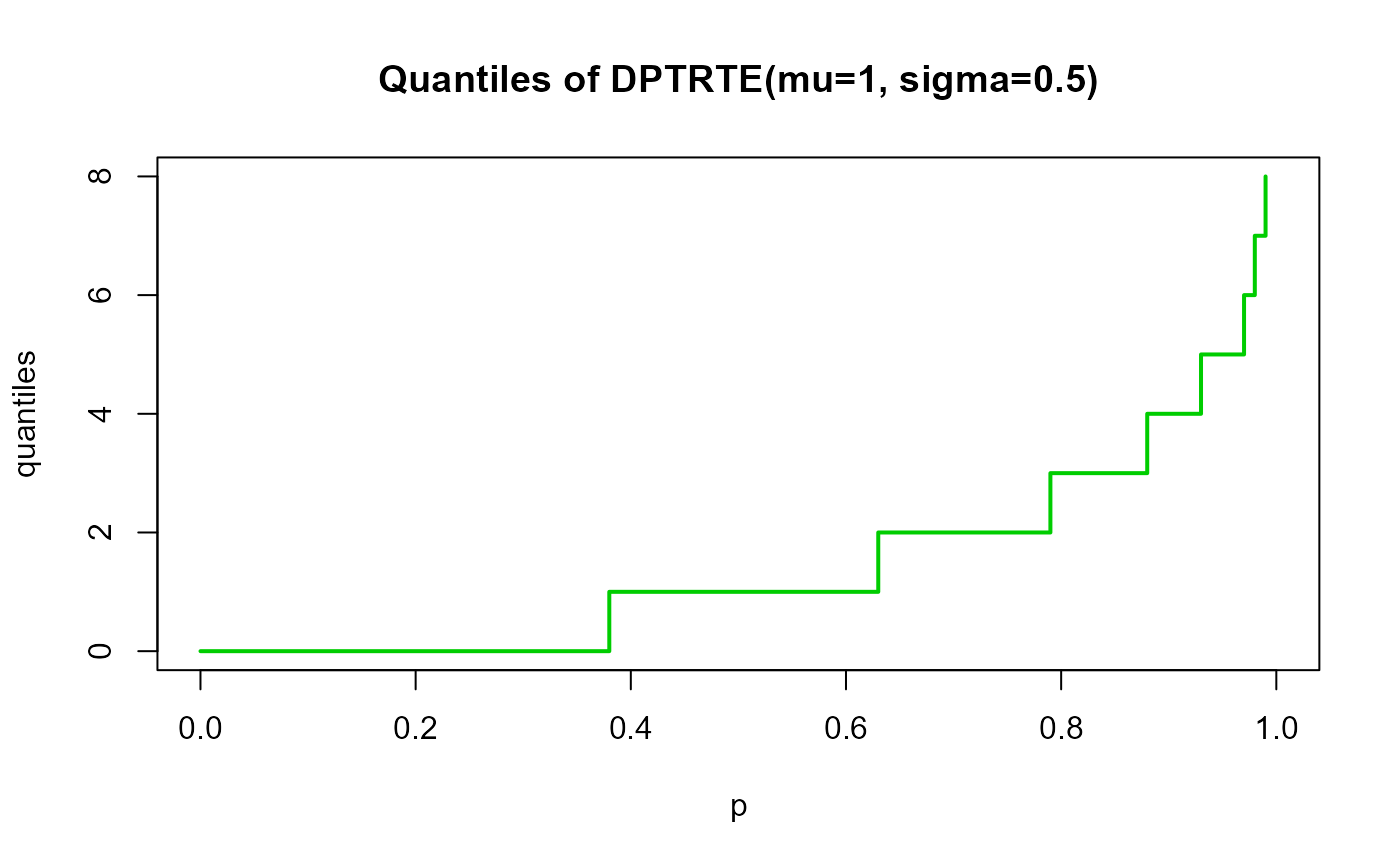
 # Example 4
# Checking the quantile function
mu <- 1
sigma <- 0.5
p <- seq(from=0, to=1, by=0.01)
qxx <- qPTRTE(p=p, mu=mu, sigma=sigma, lower.tail=TRUE, log.p=FALSE)
plot(p, qxx, type="s", lwd=2, col="green3", ylab="quantiles",
main="Quantiles of DPTRTE(mu=1, sigma=0.5)")
# Example 4
# Checking the quantile function
mu <- 1
sigma <- 0.5
p <- seq(from=0, to=1, by=0.01)
qxx <- qPTRTE(p=p, mu=mu, sigma=sigma, lower.tail=TRUE, log.p=FALSE)
plot(p, qxx, type="s", lwd=2, col="green3", ylab="quantiles",
main="Quantiles of DPTRTE(mu=1, sigma=0.5)")