These functions define the density, distribution function, quantile function and random generation for the Poisson-generalised Lindley in second parametrization with parameters \(\mu\) (as mean) and \(\sigma\).
dNPGL2(x, mu = 2, sigma = 2, log = FALSE)

pNPGL2(q, mu = 2, sigma = 2, lower.tail = TRUE, log.p = FALSE)

rNPGL2(n, mu = 2, sigma = 2)

qNPGL2(p, mu = 2, sigma = 2, lower.tail = TRUE, log.p = FALSE)
Arguments
- x, q
vector of (non-negative integer) quantiles.
- mu
vector of the mu parameter.
- sigma
vector of the sigma parameter.
- log, log.p
logical; if TRUE, probabilities p are given as log(p).
- lower.tail
logical; if TRUE (default), probabilities are \(P[X <= x]\), otherwise, \(P[X > x]\).
- n
number of random values to return.
- p
vector of probabilities.
Value
dNPGL2 gives the density, pNPGL2 gives the distribution
function, qNPGL2 gives the quantile function, rNPGL2
generates random deviates.
Details
The Poisson-generalised Lindley distribution with parameters \(\mu\) and \(\sigma\) has support \(x = 0, 1, 2, \ldots\) and probability mass function given by
Note: in this implementation the parameter \(\mu\) is the mean of the distribution and \(\sigma\) (equivalent to \(\alpha\) in the original NPGL parametrization).
References
Altun, E. A new two-parameter discrete poisson-generalized Lindley distribution with properties and applications to healthcare data sets. Comput Stat 36, 2841–2861 (2021). https://doi.org/10.1007/s00180-021-01097-0
Examples
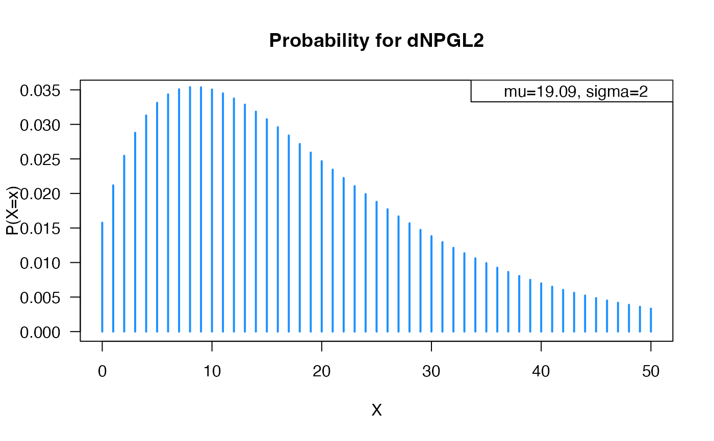
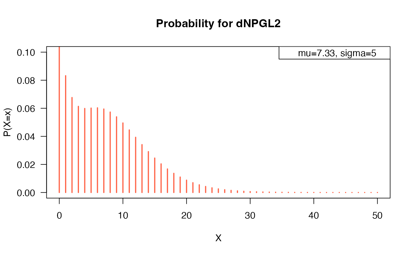
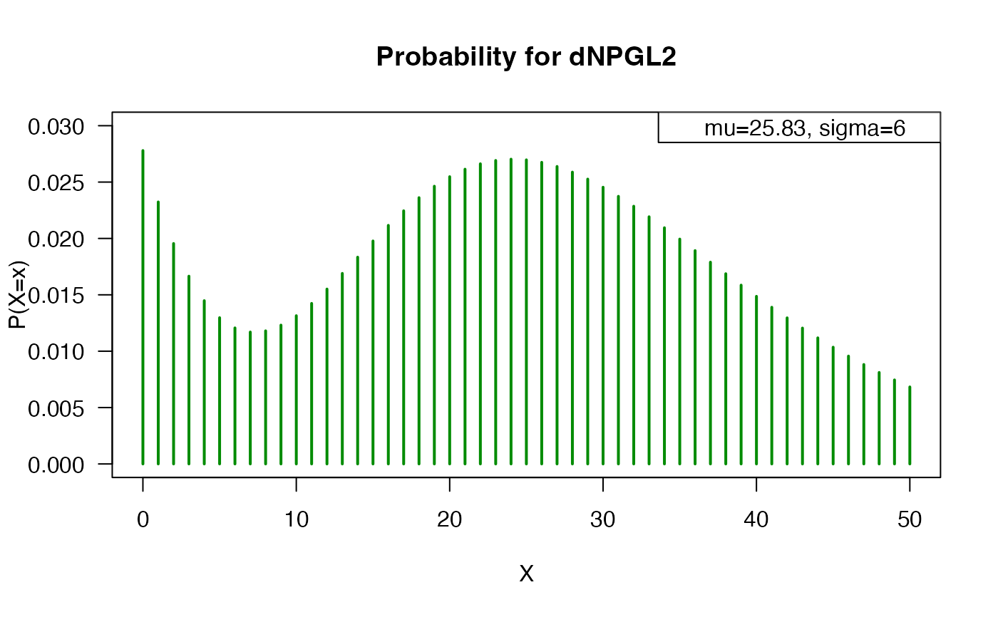
# Example 1
# Plotting the mass function for different parameter values
# Original parameters and their corresponding means
casos <- data.frame(
mu_orig = c(0.1, 0.5, 0.2, 20),
sigma = c(2, 5, 6, 2)
)
casos$mu_mean <- (casos$sigma + casos$mu_orig) /
(casos$mu_orig * (1 + casos$mu_orig))
x_max <- 50
probs1 <- dNPGL2(x=0:x_max, mu=casos$mu_mean[1], sigma=casos$sigma[1])
probs2 <- dNPGL2(x=0:x_max, mu=casos$mu_mean[2], sigma=casos$sigma[2])
probs3 <- dNPGL2(x=0:x_max, mu=casos$mu_mean[3], sigma=casos$sigma[3])
probs4 <- dNPGL2(x=0:x_max, mu=casos$mu_mean[4], sigma=casos$sigma[4])
plot(x = 0:x_max, y = probs1, type = "h", lwd = 2, col = "dodgerblue", las = 1,
ylab = "P(X=x)", xlab = "X", main = "Probability for dNPGL2",
ylim = c(0, 0.035))
legend("topright", legend = paste0("mu=", round(casos$mu_mean[1], 2),
", sigma=", casos$sigma[1]))
 plot(x = 0:x_max, y = probs2, type = "h", lwd = 2, col = "tomato", las = 1,
ylab = "P(X=x)", xlab = "X", main = "Probability for dNPGL2",
ylim = c(0, 0.1))
legend("topright", legend = paste0("mu=", round(casos$mu_mean[2], 2),
", sigma=", casos$sigma[2]))
plot(x = 0:x_max, y = probs2, type = "h", lwd = 2, col = "tomato", las = 1,
ylab = "P(X=x)", xlab = "X", main = "Probability for dNPGL2",
ylim = c(0, 0.1))
legend("topright", legend = paste0("mu=", round(casos$mu_mean[2], 2),
", sigma=", casos$sigma[2]))
 plot(x = 0:x_max, y = probs3, type = "h", lwd = 2, col = "green4", las = 1,
ylab = "P(X=x)", xlab = "X", main = "Probability for dNPGL2",
ylim = c(0, 0.03))
legend("topright", legend = paste0("mu=", round(casos$mu_mean[3], 2),
", sigma=", casos$sigma[3]))
plot(x = 0:x_max, y = probs3, type = "h", lwd = 2, col = "green4", las = 1,
ylab = "P(X=x)", xlab = "X", main = "Probability for dNPGL2",
ylim = c(0, 0.03))
legend("topright", legend = paste0("mu=", round(casos$mu_mean[3], 2),
", sigma=", casos$sigma[3]))
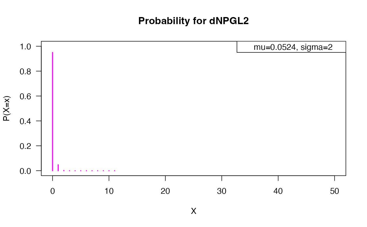
 plot(x = 0:x_max, y = probs4, type = "h", lwd = 2, col = "magenta", las = 1,
ylab = "P(X=x)", xlab = "X", main = "Probability for dNPGL2",
ylim = c(0, 1))
legend("topright", legend = paste0("mu=", round(casos$mu_mean[4], 4),
", sigma=", casos$sigma[4]))
plot(x = 0:x_max, y = probs4, type = "h", lwd = 2, col = "magenta", las = 1,
ylab = "P(X=x)", xlab = "X", main = "Probability for dNPGL2",
ylim = c(0, 1))
legend("topright", legend = paste0("mu=", round(casos$mu_mean[4], 4),
", sigma=", casos$sigma[4]))
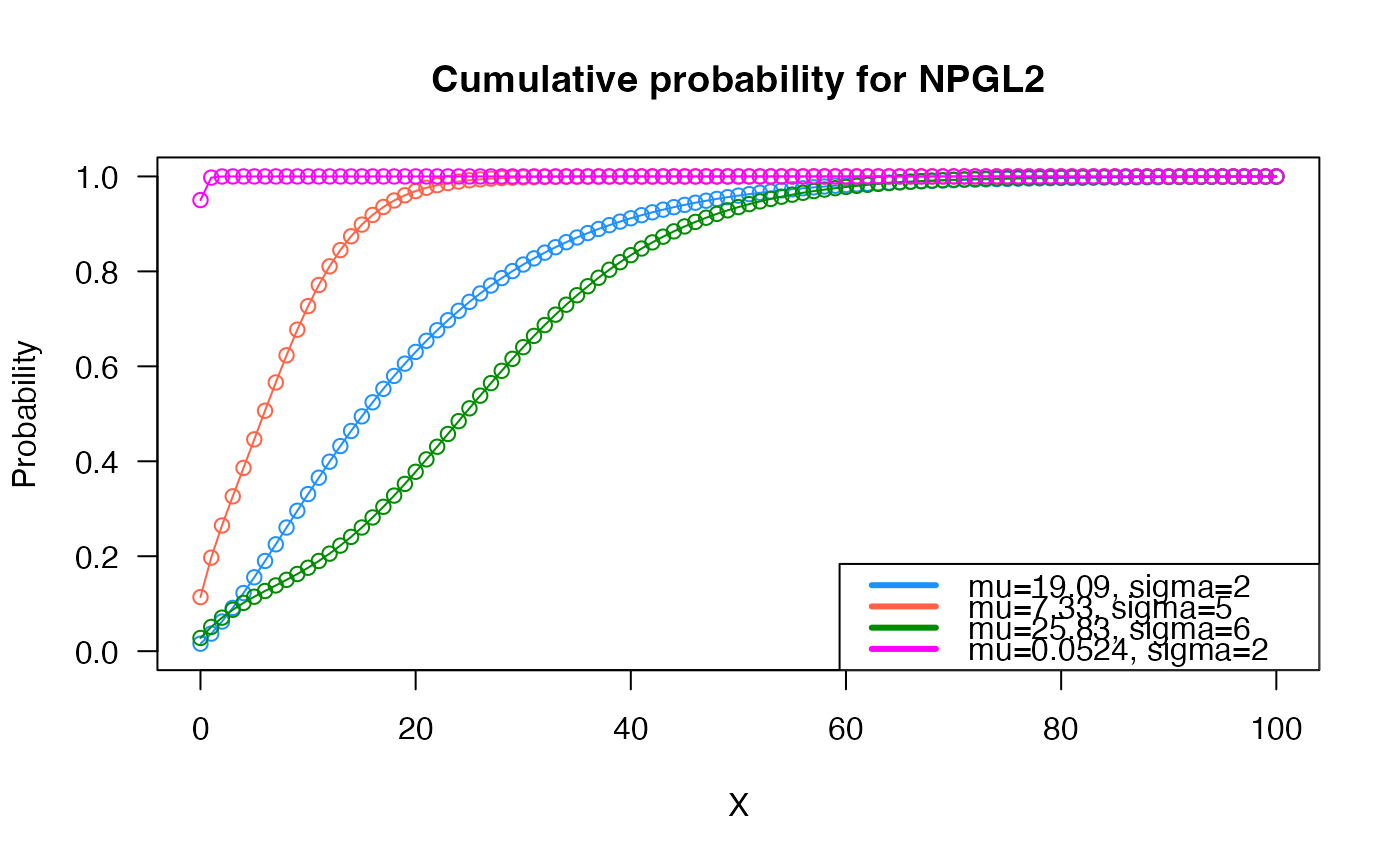
 # Example 2
# Checking if the cumulative curves converge to 1
x_max <- 100
cumulative_probs1 <- pNPGL2(q = 0:x_max, mu = casos$mu_mean[1], sigma = casos$sigma[1])
cumulative_probs2 <- pNPGL2(q = 0:x_max, mu = casos$mu_mean[2], sigma = casos$sigma[2])
cumulative_probs3 <- pNPGL2(q = 0:x_max, mu = casos$mu_mean[3], sigma = casos$sigma[3])
cumulative_probs4 <- pNPGL2(q = 0:x_max, mu = casos$mu_mean[4], sigma = casos$sigma[4])
plot(x = 0:x_max, y = cumulative_probs1, col = "dodgerblue",
type = "o", las = 1, ylim = c(0, 1),
main = "Cumulative probability for NPGL2",
xlab = "X", ylab = "Probability")
points(x = 0:x_max, y = cumulative_probs2, type = "o", col = "tomato")
points(x = 0:x_max, y = cumulative_probs3, type = "o", col = "green4")
points(x = 0:x_max, y = cumulative_probs4, type = "o", col = "magenta")
legend("bottomright",
col = c("dodgerblue", "tomato", "green4", "magenta"), lwd = 3,
legend = c(
paste0("mu=", round(casos$mu_mean[1], 2), ", sigma=", casos$sigma[1]),
paste0("mu=", round(casos$mu_mean[2], 2), ", sigma=", casos$sigma[2]),
paste0("mu=", round(casos$mu_mean[3], 2), ", sigma=", casos$sigma[3]),
paste0("mu=", round(casos$mu_mean[4], 4), ", sigma=", casos$sigma[4])
))
# Example 2
# Checking if the cumulative curves converge to 1
x_max <- 100
cumulative_probs1 <- pNPGL2(q = 0:x_max, mu = casos$mu_mean[1], sigma = casos$sigma[1])
cumulative_probs2 <- pNPGL2(q = 0:x_max, mu = casos$mu_mean[2], sigma = casos$sigma[2])
cumulative_probs3 <- pNPGL2(q = 0:x_max, mu = casos$mu_mean[3], sigma = casos$sigma[3])
cumulative_probs4 <- pNPGL2(q = 0:x_max, mu = casos$mu_mean[4], sigma = casos$sigma[4])
plot(x = 0:x_max, y = cumulative_probs1, col = "dodgerblue",
type = "o", las = 1, ylim = c(0, 1),
main = "Cumulative probability for NPGL2",
xlab = "X", ylab = "Probability")
points(x = 0:x_max, y = cumulative_probs2, type = "o", col = "tomato")
points(x = 0:x_max, y = cumulative_probs3, type = "o", col = "green4")
points(x = 0:x_max, y = cumulative_probs4, type = "o", col = "magenta")
legend("bottomright",
col = c("dodgerblue", "tomato", "green4", "magenta"), lwd = 3,
legend = c(
paste0("mu=", round(casos$mu_mean[1], 2), ", sigma=", casos$sigma[1]),
paste0("mu=", round(casos$mu_mean[2], 2), ", sigma=", casos$sigma[2]),
paste0("mu=", round(casos$mu_mean[3], 2), ", sigma=", casos$sigma[3]),
paste0("mu=", round(casos$mu_mean[4], 4), ", sigma=", casos$sigma[4])
))
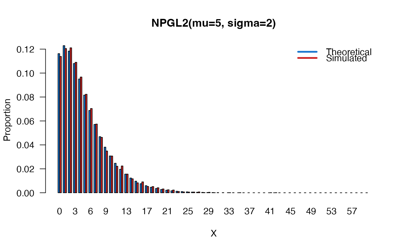
 # Example 3
# Comparing the random generator output with
# the theoretical probabilities
x_max <- 60
mu <- 5
sigma <- 2
probs1 <- dNPGL2(x = 0:x_max, mu = mu, sigma = sigma)
names(probs1) <- 0:x_max
set.seed(123)
x <- rNPGL2(n = 10000, mu = mu, sigma = sigma)
probs2 <- prop.table(table(x))
cn <- union(names(probs1), names(probs2))
height <- rbind(probs1[cn], probs2[cn])
mp <- barplot(height, beside = TRUE, names.arg = cn,
col = c("dodgerblue3", "firebrick3"), las = 1,
xlab = "X", ylab = "Proportion",
main = paste0("NPGL2(mu=", mu, ", sigma=", sigma, ")"))
legend("topright",
legend = c("Theoretical", "Simulated"),
bty = "n", lwd = 3,
col = c("dodgerblue3", "firebrick3"), lty = 1)
# Example 3
# Comparing the random generator output with
# the theoretical probabilities
x_max <- 60
mu <- 5
sigma <- 2
probs1 <- dNPGL2(x = 0:x_max, mu = mu, sigma = sigma)
names(probs1) <- 0:x_max
set.seed(123)
x <- rNPGL2(n = 10000, mu = mu, sigma = sigma)
probs2 <- prop.table(table(x))
cn <- union(names(probs1), names(probs2))
height <- rbind(probs1[cn], probs2[cn])
mp <- barplot(height, beside = TRUE, names.arg = cn,
col = c("dodgerblue3", "firebrick3"), las = 1,
xlab = "X", ylab = "Proportion",
main = paste0("NPGL2(mu=", mu, ", sigma=", sigma, ")"))
legend("topright",
legend = c("Theoretical", "Simulated"),
bty = "n", lwd = 3,
col = c("dodgerblue3", "firebrick3"), lty = 1)
 # Example 4
# Checking the quantile function
mu <- 5
sigma <- 2
p <- seq(from = 0, to = 1, by = 0.01)
qxx <- qNPGL2(p = p, mu = mu, sigma = sigma, lower.tail = TRUE, log.p = FALSE)
plot(p, qxx, type = "s", lwd = 2, col = "green3", ylab = "quantiles",
main = paste0("Quantiles of NPGL2(mu=", mu, ", sigma=", sigma, ")"))
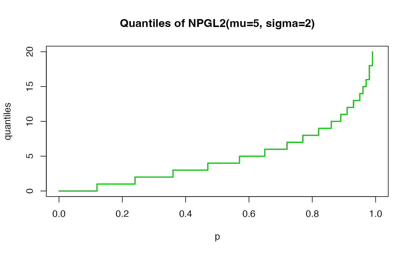
# Example 4
# Checking the quantile function
mu <- 5
sigma <- 2
p <- seq(from = 0, to = 1, by = 0.01)
qxx <- qNPGL2(p = p, mu = mu, sigma = sigma, lower.tail = TRUE, log.p = FALSE)
plot(p, qxx, type = "s", lwd = 2, col = "green3", ylab = "quantiles",
main = paste0("Quantiles of NPGL2(mu=", mu, ", sigma=", sigma, ")"))