These functions define the density, distribution function, quantile function and random generation for the discrete power-Ailamujia distribution with parameters \(\mu\) and \(\sigma\).
dDsPA(x, mu, sigma, log = FALSE)

pDsPA(q, mu, sigma, lower.tail = TRUE, log.p = FALSE)

qDsPA(p, mu = 1, sigma = 1, lower.tail = TRUE, log.p = FALSE)

rDsPA(n, mu, sigma)
Arguments
- x, q
vector of (non-negative integer) quantiles.
- mu
vector of the mu parameter.
- sigma
vector of the sigma parameter.
- log, log.p
logical; if TRUE, probabilities p are given as log(p).
- lower.tail
logical; if TRUE (default), probabilities are \(P[X <= x]\), otherwise, \(P[X > x]\).
- p
vector of probabilities.
- n
number of random values to return.
Value
dDsPA gives the density, pDsPA gives the distribution
function, qDsPA gives the quantile function.
Details
The DsPA distribution with parameters \(\mu\) and \(\sigma\) has a support 0, 1, 2, ...
Note:in this implementation we changed the original parameters \(\beta\) and \(\lambda\) for \(\mu\) and \(\sigma\) respectively, we did it to implement this distribution within gamlss framework.
References
Alghamdi, A. S., Ahsan-ul-Haq, M., Babar, A., Aljohani, H. M., Afify, A. Z., & Cell, Q. E. (2022). The discrete power-Ailamujia distribution: properties, inference, and applications. AIMS Math, 7(5), 8344-8360.
See also
DsPA.
Examples
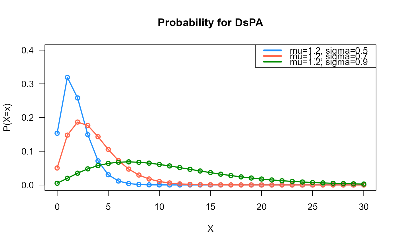
# Example 1
# Plotting the mass function for different parameter values
x_max <- 30
probs1 <- dDsPA(x=0:x_max, mu=1.2, sigma=0.5)
probs2 <- dDsPA(x=0:x_max, mu=1.2, sigma=0.7)
probs3 <- dDsPA(x=0:x_max, mu=1.2, sigma=0.9)
# To plot the first k values
plot(x=0:x_max, y=probs1, type="o", lwd=2, col="dodgerblue", las=1,
ylab="P(X=x)", xlab="X", main="Probability for DsPA",
ylim=c(0, 0.40))
points(x=0:x_max, y=probs2, type="o", lwd=2, col="tomato")
points(x=0:x_max, y=probs3, type="o", lwd=2, col="green4")
legend("topright", col=c("dodgerblue", "tomato", "green4"), lwd=3,
legend=c("mu=1.2, sigma=0.5",
"mu=1.2, sigma=0.7",
"mu=1.2, sigma=0.9"))
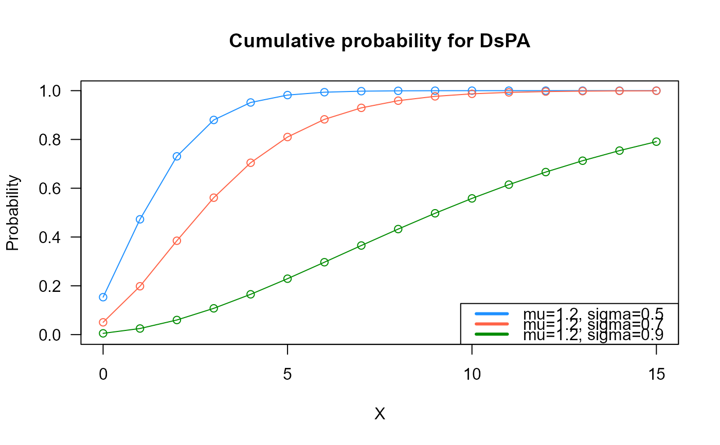
 # Example 2
# Checking if the cumulative curves converge to 1
x_max <- 15
cumulative_probs1 <- pDsPA(q=0:x_max, mu=1.2, sigma=0.5)
cumulative_probs2 <- pDsPA(q=0:x_max, mu=1.2, sigma=0.7)
cumulative_probs3 <- pDsPA(q=0:x_max, mu=1.2, sigma=0.9)
plot(x=0:x_max, y=cumulative_probs1, col="dodgerblue",
type="o", las=1, ylim=c(0, 1),
main="Cumulative probability for DsPA",
xlab="X", ylab="Probability")
points(x=0:x_max, y=cumulative_probs2, type="o", col="tomato")
points(x=0:x_max, y=cumulative_probs3, type="o", col="green4")
legend("bottomright", col=c("dodgerblue", "tomato", "green4"), lwd=3,
legend=c("mu=1.2, sigma=0.5",
"mu=1.2, sigma=0.7",
"mu=1.2, sigma=0.9"))
# Example 2
# Checking if the cumulative curves converge to 1
x_max <- 15
cumulative_probs1 <- pDsPA(q=0:x_max, mu=1.2, sigma=0.5)
cumulative_probs2 <- pDsPA(q=0:x_max, mu=1.2, sigma=0.7)
cumulative_probs3 <- pDsPA(q=0:x_max, mu=1.2, sigma=0.9)
plot(x=0:x_max, y=cumulative_probs1, col="dodgerblue",
type="o", las=1, ylim=c(0, 1),
main="Cumulative probability for DsPA",
xlab="X", ylab="Probability")
points(x=0:x_max, y=cumulative_probs2, type="o", col="tomato")
points(x=0:x_max, y=cumulative_probs3, type="o", col="green4")
legend("bottomright", col=c("dodgerblue", "tomato", "green4"), lwd=3,
legend=c("mu=1.2, sigma=0.5",
"mu=1.2, sigma=0.7",
"mu=1.2, sigma=0.9"))
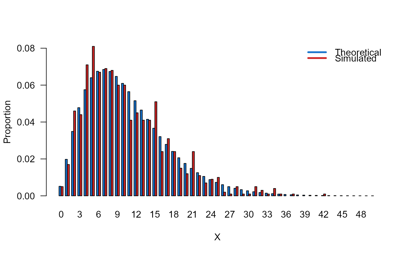
 # Example 3
# Comparing the random generator output with
# the theoretical probabilities
x_max <- 50
probs1 <- dDsPA(x=0:x_max, mu=1.2, sigma=0.9)
names(probs1) <- 0:x_max
x <- rDsPA(n=1000, mu=1.2, sigma=0.9)
probs2 <- prop.table(table(x))
cn <- union(names(probs1), names(probs2))
height <- rbind(probs1[cn], probs2[cn])
mp <- barplot(height, beside=TRUE, names.arg=cn,
col=c("dodgerblue3","firebrick3"), las=1,
xlab="X", ylab="Proportion")
legend("topright",
legend=c("Theoretical", "Simulated"),
bty="n", lwd=3,
col=c("dodgerblue3","firebrick3"), lty=1)
# Example 3
# Comparing the random generator output with
# the theoretical probabilities
x_max <- 50
probs1 <- dDsPA(x=0:x_max, mu=1.2, sigma=0.9)
names(probs1) <- 0:x_max
x <- rDsPA(n=1000, mu=1.2, sigma=0.9)
probs2 <- prop.table(table(x))
cn <- union(names(probs1), names(probs2))
height <- rbind(probs1[cn], probs2[cn])
mp <- barplot(height, beside=TRUE, names.arg=cn,
col=c("dodgerblue3","firebrick3"), las=1,
xlab="X", ylab="Proportion")
legend("topright",
legend=c("Theoretical", "Simulated"),
bty="n", lwd=3,
col=c("dodgerblue3","firebrick3"), lty=1)
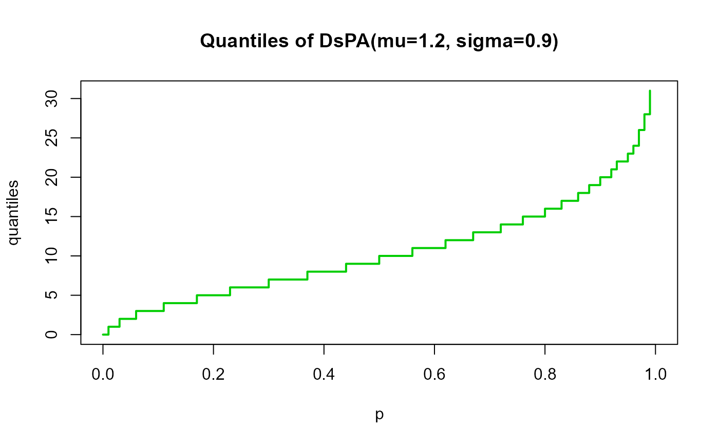
 # Example 4
# Checking the quantile function
mu <- 1.2
sigma <- 0.9
p <- seq(from=0, to=1, by=0.01)
qxx <- qDsPA(p=p, mu=mu, sigma=sigma,
lower.tail=TRUE, log.p=FALSE)
plot(p, qxx, type="s", lwd=2, col="green3", ylab="quantiles",
main="Quantiles of DsPA(mu=1.2, sigma=0.9)")
# Example 4
# Checking the quantile function
mu <- 1.2
sigma <- 0.9
p <- seq(from=0, to=1, by=0.01)
qxx <- qDsPA(p=p, mu=mu, sigma=sigma,
lower.tail=TRUE, log.p=FALSE)
plot(p, qxx, type="s", lwd=2, col="green3", ylab="quantiles",
main="Quantiles of DsPA(mu=1.2, sigma=0.9)")