These functions define the density, distribution function, quantile function and random generation for the Discrete Perks, DPERKS(), distribution with parameters \(\mu\) and \(\sigma\).
dDPERKS(x, mu = 0.5, sigma = 0.5, log = FALSE)

pDPERKS(q, mu = 0.5, sigma = 0.5, lower.tail = TRUE, log.p = FALSE)

rDPERKS(n, mu = 0.5, sigma = 0.5)

qDPERKS(p, mu = 0.5, sigma = 0.5, lower.tail = TRUE, log.p = FALSE)
Arguments
- x, q
vector of (non-negative integer) quantiles.
- mu
vector of the mu parameter.
- sigma
vector of the sigma parameter.
- log, log.p
logical; if TRUE, probabilities p are given as log(p).
- lower.tail
logical; if TRUE (default), probabilities are \(P[X <= x]\), otherwise, \(P[X > x]\).
- n
number of random values to return.
- p
vector of probabilities.
Value
dDPERKS gives the density, pDPERKS gives the distribution
function, qDPERKS gives the quantile function, rDPERKS
generates random deviates.
Details
The discrete Perks distribution with parameters \(\mu > 0\) and \(\sigma > 0\) has a support 0, 1, 2, ... and density given by
\(f(x | \mu, \sigma) = \frac{\mu(1+\mu)(e^\sigma-1)e^{\sigma x}}{(1+\mu e^{\sigma x})(1+\mu e^{\sigma(x+1)})} \)
Note: in this implementation we changed the original parameters \(\lambda\) for \(\mu\) and \(\beta\) for \(\sigma\), we did it to implement this distribution within gamlss framework.
References
Tyagi, A., Choudhary, N., & Singh, B. (2020). A new discrete distribution: Theory and applications to discrete failure lifetime and count data. J. Appl. Probab. Statist, 15, 117-143.
See also
Examples
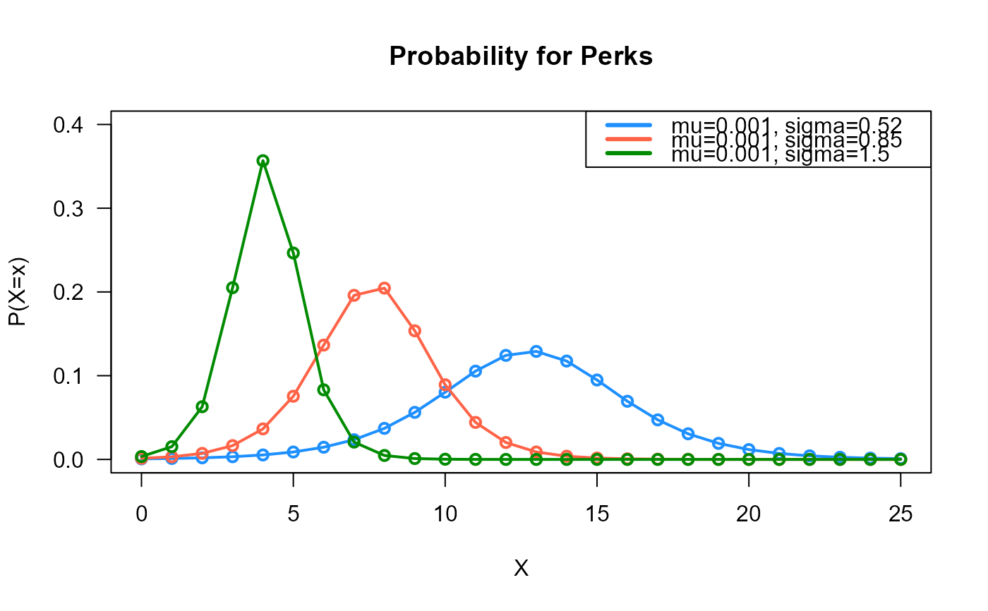
# Example 1
# Plotting the mass function for different parameter values
x_max <- 25
probs1 <- dDPERKS(x=0:x_max, mu=0.001, sigma=0.52)
probs2 <- dDPERKS(x=0:x_max, mu=0.001, sigma=0.85)
probs3 <- dDPERKS(x=0:x_max, mu=0.001, sigma=1.5)
# To plot the first k values
plot(x=0:x_max, y=probs1, type="o", lwd=2, col="green4", las=1,
ylab="P(X=x)", xlab="X", main="Probability for DPERKS",
ylim=c(0, 0.40))
points(x=0:x_max, y=probs2, type="o", lwd=2, col="tomato")
points(x=0:x_max, y=probs3, type="o", lwd=2, col="black")
legend("topright", col=c("green4", "tomato", "black"), lwd=3,
legend=c("mu=0.001, sigma=0.52 ",
"mu=0.001, sigma=0.85",
"mu=0.001, sigma=1.5"))
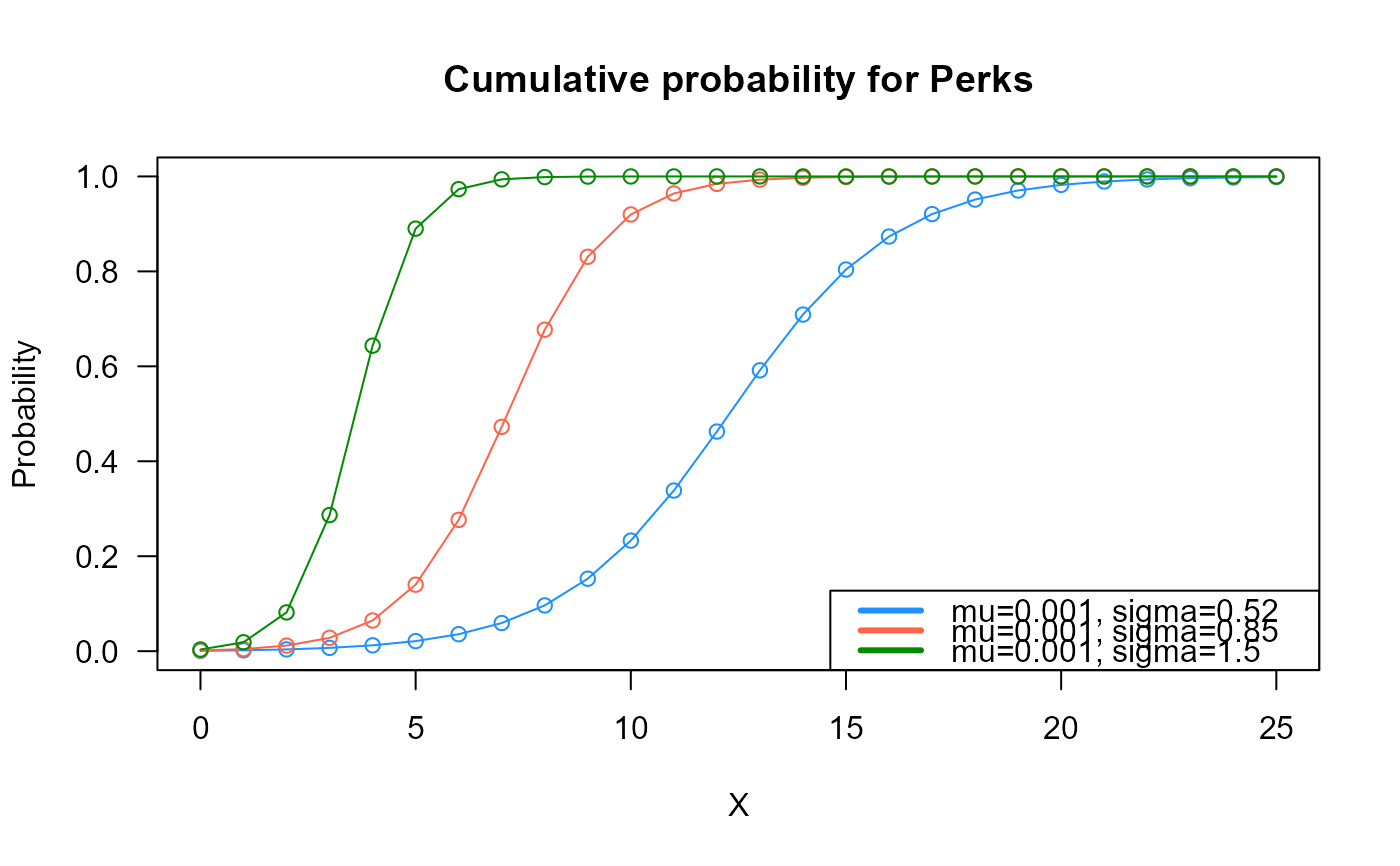
 # Example 2
# Checking if the cumulative curves converge to 1
x_max <- 25
cumulative_probs1 <- pDPERKS(q=0:x_max, mu=0.001, sigma=0.52)
cumulative_probs2 <- pDPERKS(q=0:x_max, mu=0.001, sigma=0.85)
cumulative_probs3 <- pDPERKS(q=0:x_max, mu=0.001, sigma=1.5)
plot(x=0:x_max, y=cumulative_probs1, col="green4",
type="o", las=1, ylim=c(0, 1),
main="Cumulative probability for DPERKS",
xlab="X", ylab="Probability")
points(x=0:x_max, y=cumulative_probs2, type="o", col="tomato")
points(x=0:x_max, y=cumulative_probs3, type="o", col="black")
legend("bottomright", col=c("green4", "tomato", "black"), lwd=3,
legend=c("mu=0.001, sigma=0.52 ",
"mu=0.001, sigma=0.85",
"mu=0.001, sigma=1.5"))
# Example 2
# Checking if the cumulative curves converge to 1
x_max <- 25
cumulative_probs1 <- pDPERKS(q=0:x_max, mu=0.001, sigma=0.52)
cumulative_probs2 <- pDPERKS(q=0:x_max, mu=0.001, sigma=0.85)
cumulative_probs3 <- pDPERKS(q=0:x_max, mu=0.001, sigma=1.5)
plot(x=0:x_max, y=cumulative_probs1, col="green4",
type="o", las=1, ylim=c(0, 1),
main="Cumulative probability for DPERKS",
xlab="X", ylab="Probability")
points(x=0:x_max, y=cumulative_probs2, type="o", col="tomato")
points(x=0:x_max, y=cumulative_probs3, type="o", col="black")
legend("bottomright", col=c("green4", "tomato", "black"), lwd=3,
legend=c("mu=0.001, sigma=0.52 ",
"mu=0.001, sigma=0.85",
"mu=0.001, sigma=1.5"))
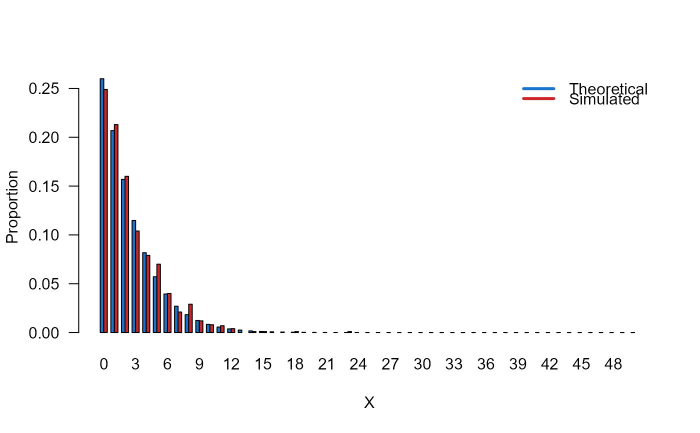
 # Example 3
# Comparing the random generator output with the theoretical probabilities
x_max <- 20
mu <- 2.5
sigma <- 0.4
probs1 <- dDPERKS(x=0:x_max, mu=mu, sigma=sigma)
names(probs1) <- 0:x_max
x <- rDPERKS(n=10000, mu=mu, sigma=sigma)
probs2 <- prop.table(table(x))
cn <- union(names(probs1), names(probs2))
height <- rbind(probs1[cn], probs2[cn])
nombres <- cn
mp <- barplot(height, beside = TRUE, names.arg = nombres,
col=c("dodgerblue3","firebrick3"), las=1,
xlab="X", ylab="Proportion")
legend("topright",
legend=c("Theoretical", "Simulated"),
bty="n", lwd=3,
col=c("dodgerblue3","firebrick3"), lty=1)
# Example 3
# Comparing the random generator output with the theoretical probabilities
x_max <- 20
mu <- 2.5
sigma <- 0.4
probs1 <- dDPERKS(x=0:x_max, mu=mu, sigma=sigma)
names(probs1) <- 0:x_max
x <- rDPERKS(n=10000, mu=mu, sigma=sigma)
probs2 <- prop.table(table(x))
cn <- union(names(probs1), names(probs2))
height <- rbind(probs1[cn], probs2[cn])
nombres <- cn
mp <- barplot(height, beside = TRUE, names.arg = nombres,
col=c("dodgerblue3","firebrick3"), las=1,
xlab="X", ylab="Proportion")
legend("topright",
legend=c("Theoretical", "Simulated"),
bty="n", lwd=3,
col=c("dodgerblue3","firebrick3"), lty=1)
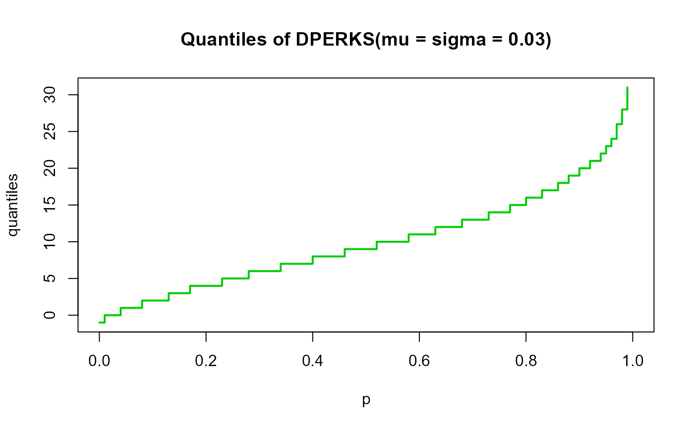
 # Example 4
# Checking the quantile function
mu <- 0.2
sigma <- 0.2
p <- seq(from=0, to=1, by=0.01)
qxx <- qDPERKS(p=p, mu=mu, sigma=sigma, lower.tail=TRUE, log.p=FALSE)
plot(p, qxx, type="s", lwd=2, col="green3", ylab="quantiles",
main="Quantiles of DPERKS(mu = sigma = 0.2)")
# Example 4
# Checking the quantile function
mu <- 0.2
sigma <- 0.2
p <- seq(from=0, to=1, by=0.01)
qxx <- qDPERKS(p=p, mu=mu, sigma=sigma, lower.tail=TRUE, log.p=FALSE)
plot(p, qxx, type="s", lwd=2, col="green3", ylab="quantiles",
main="Quantiles of DPERKS(mu = sigma = 0.2)")