These functions define the density, distribution function, quantile function and random generation for the Discrete Lindley distribution with parameter \(\mu\).
dDLD(x, mu, log = FALSE)

pDLD(q, mu, lower.tail = TRUE, log.p = FALSE)

qDLD(p, mu, lower.tail = TRUE, log.p = FALSE)

rDLD(n, mu = 0.5)
Arguments
- x, q
vector of (non-negative integer) quantiles.
- mu
vector of positive values of this parameter.
- log, log.p
logical; if TRUE, probabilities p are given as log(p).
- lower.tail
logical; if TRUE (default), probabilities are \(P[X <= x]\), otherwise, \(P[X > x]\).
- p
vector of probabilities.
- n
number of random values to return.
Value
dDLD gives the density, pDLD gives the distribution
function, qDLD gives the quantile function, rDLD
generates random deviates.
Details
The Discrete Lindley distribution with parameters \(\mu\) has a support 0, 1, 2, ... and density given by
\(f(x | \mu) = \frac{e^{-\mu x}}{1 + \mu} \left[ \mu(1 - 2e^{-\mu}) + (1- e^{-\mu})(1+\mu x)\right]\)
Note: in this implementation we changed the original parameters \(\theta\) for \(\mu\), we did it to implement this distribution within gamlss framework.
References
Bakouch, H. S., Jazi, M. A., & Nadarajah, S. (2014). A new discrete distribution. Statistics, 48(1), 200-240.
See also
DLD.
Examples
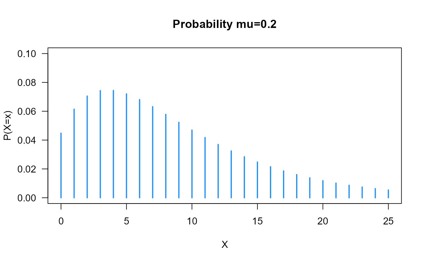
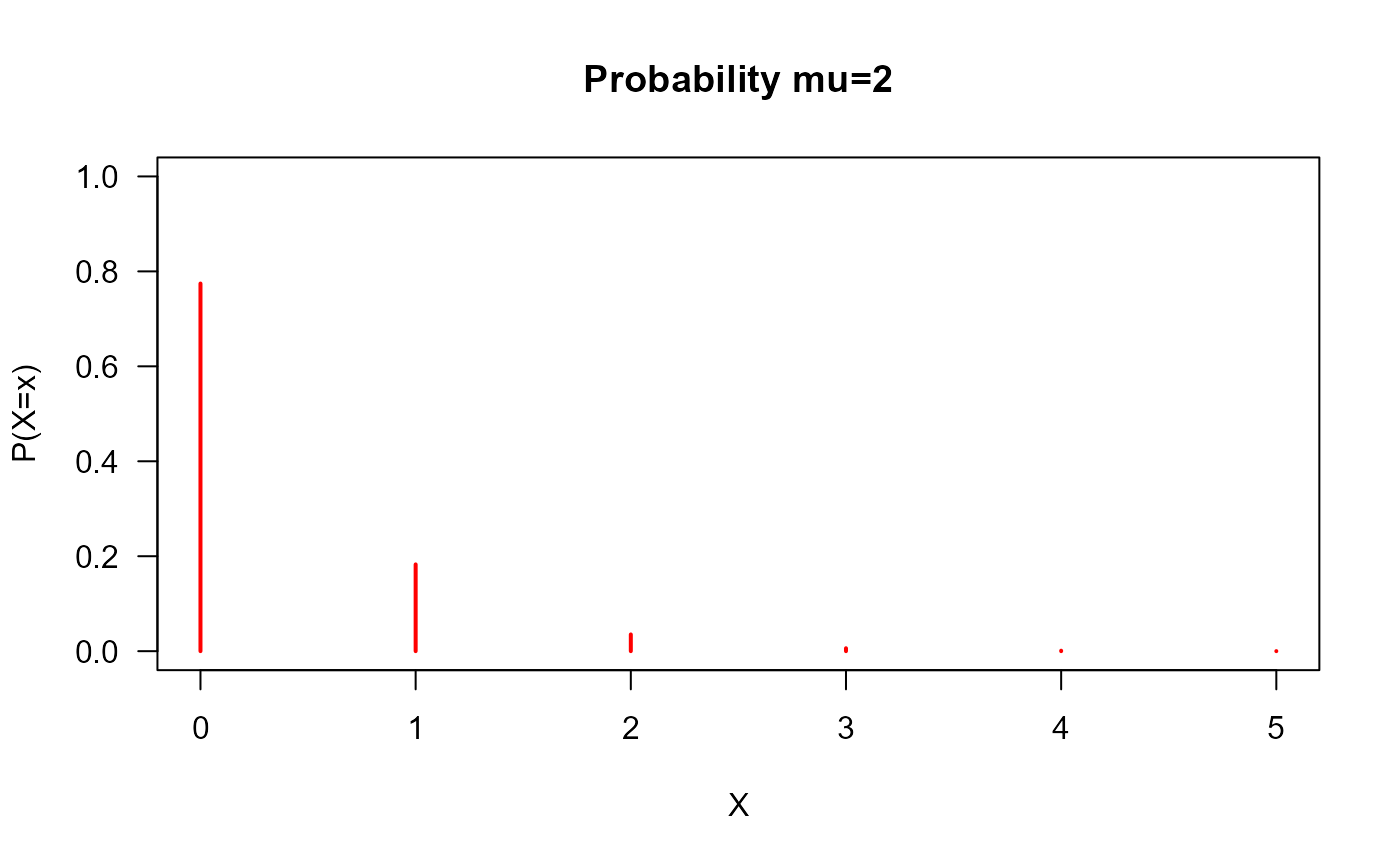
# Example 1
# Plotting the mass function for different parameter values
plot(x=0:25, y=dDLD(x=0:25, mu=0.2),
type="h", lwd=2, col="dodgerblue", las=1,
ylab="P(X=x)", xlab="X", ylim=c(0, 0.1),
main="Probability mu=0.2")
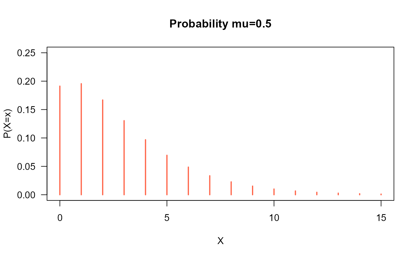
 plot(x=0:15, y=dDLD(x=0:15, mu=0.5),
type="h", lwd=2, col="tomato", las=1,
ylab="P(X=x)", xlab="X", ylim=c(0, 0.25),
main="Probability mu=0.5")
plot(x=0:15, y=dDLD(x=0:15, mu=0.5),
type="h", lwd=2, col="tomato", las=1,
ylab="P(X=x)", xlab="X", ylim=c(0, 0.25),
main="Probability mu=0.5")
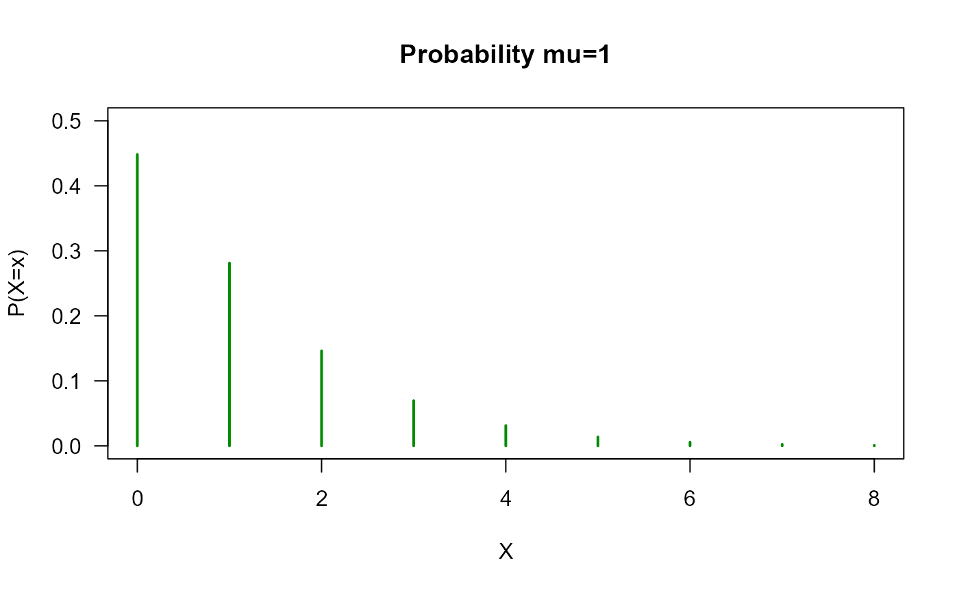
 plot(x=0:8, y=dDLD(x=0:8, mu=1),
type="h", lwd=2, col="green4", las=1,
ylab="P(X=x)", xlab="X", ylim=c(0, 0.5),
main="Probability mu=1")
plot(x=0:8, y=dDLD(x=0:8, mu=1),
type="h", lwd=2, col="green4", las=1,
ylab="P(X=x)", xlab="X", ylim=c(0, 0.5),
main="Probability mu=1")
 plot(x=0:5, y=dDLD(x=0:5, mu=2),
type="h", lwd=2, col="red", las=1,
ylab="P(X=x)", xlab="X", ylim=c(0, 1),
main="Probability mu=2")
plot(x=0:5, y=dDLD(x=0:5, mu=2),
type="h", lwd=2, col="red", las=1,
ylab="P(X=x)", xlab="X", ylim=c(0, 1),
main="Probability mu=2")
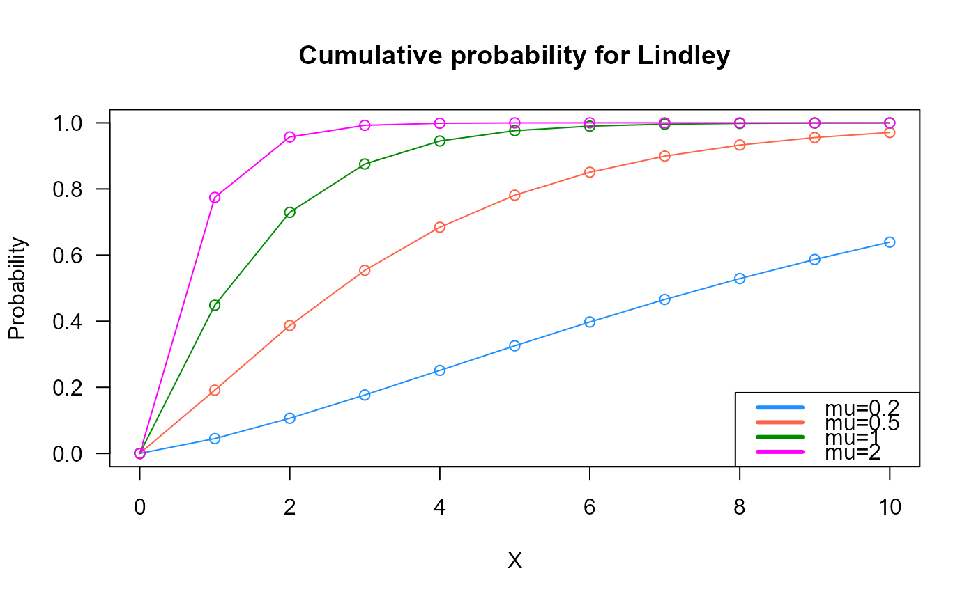
 # Example 2
# Checking if the cumulative curves converge to 1
x_max <- 10
cumulative_probs1 <- pDLD(q=0:x_max, mu=0.2)
cumulative_probs2 <- pDLD(q=0:x_max, mu=0.5)
cumulative_probs3 <- pDLD(q=0:x_max, mu=1)
cumulative_probs4 <- pDLD(q=0:x_max, mu=2)
plot(x=0:x_max, y=cumulative_probs1, col="dodgerblue",
type="o", las=1, ylim=c(0, 1),
main="Cumulative probability for Lindley",
xlab="X", ylab="Probability")
points(x=0:x_max, y=cumulative_probs2, type="o", col="tomato")
points(x=0:x_max, y=cumulative_probs3, type="o", col="green4")
points(x=0:x_max, y=cumulative_probs4, type="o", col="magenta")
legend("bottomright",
col=c("dodgerblue", "tomato", "green4", "magenta"), lwd=3,
legend=c("mu=0.2",
"mu=0.5",
"mu=1",
"mu=2"))
# Example 2
# Checking if the cumulative curves converge to 1
x_max <- 10
cumulative_probs1 <- pDLD(q=0:x_max, mu=0.2)
cumulative_probs2 <- pDLD(q=0:x_max, mu=0.5)
cumulative_probs3 <- pDLD(q=0:x_max, mu=1)
cumulative_probs4 <- pDLD(q=0:x_max, mu=2)
plot(x=0:x_max, y=cumulative_probs1, col="dodgerblue",
type="o", las=1, ylim=c(0, 1),
main="Cumulative probability for Lindley",
xlab="X", ylab="Probability")
points(x=0:x_max, y=cumulative_probs2, type="o", col="tomato")
points(x=0:x_max, y=cumulative_probs3, type="o", col="green4")
points(x=0:x_max, y=cumulative_probs4, type="o", col="magenta")
legend("bottomright",
col=c("dodgerblue", "tomato", "green4", "magenta"), lwd=3,
legend=c("mu=0.2",
"mu=0.5",
"mu=1",
"mu=2"))
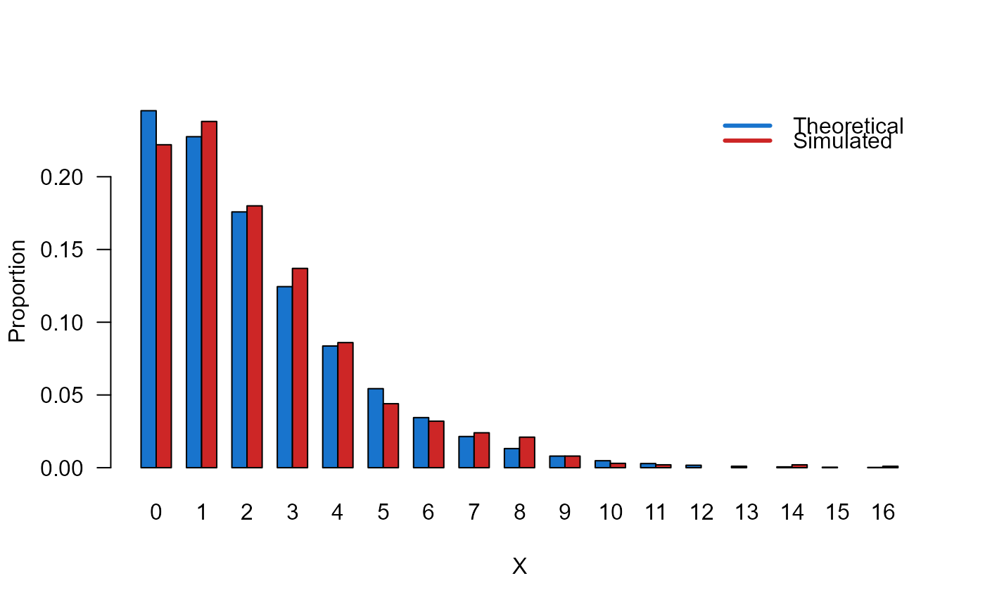
 # Example 3
# Comparing the random generator output with
# the theoretical probabilities
mu <- 0.6
x <- rDLD(n = 1000, mu = mu)
x_max <- max(x)
probs1 <- dDLD(x = 0:x_max, mu = mu)
names(probs1) <- 0:x_max
probs2 <- prop.table(table(x))
cn <- union(names(probs1), names(probs2))
height <- rbind(probs1[cn], probs2[cn])
mp <- barplot(height, beside = TRUE, names.arg = cn,
col=c("dodgerblue3","firebrick3"), las=1,
xlab="X", ylab="Proportion")
legend("topright",
legend=c("Theoretical", "Simulated"),
bty="n", lwd=3,
col=c("dodgerblue3","firebrick3"), lty=1)
# Example 3
# Comparing the random generator output with
# the theoretical probabilities
mu <- 0.6
x <- rDLD(n = 1000, mu = mu)
x_max <- max(x)
probs1 <- dDLD(x = 0:x_max, mu = mu)
names(probs1) <- 0:x_max
probs2 <- prop.table(table(x))
cn <- union(names(probs1), names(probs2))
height <- rbind(probs1[cn], probs2[cn])
mp <- barplot(height, beside = TRUE, names.arg = cn,
col=c("dodgerblue3","firebrick3"), las=1,
xlab="X", ylab="Proportion")
legend("topright",
legend=c("Theoretical", "Simulated"),
bty="n", lwd=3,
col=c("dodgerblue3","firebrick3"), lty=1)
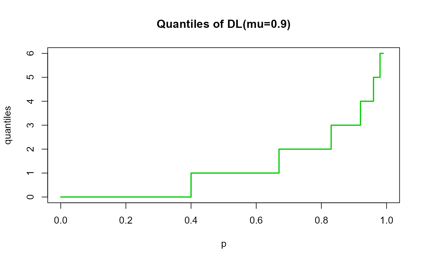
 # Example 4
# Checking the quantile function
mu <- 0.9
p <- seq(from=0, to=1, by=0.01)
qxx <- qDLD(p, mu, lower.tail = TRUE, log.p = FALSE)
plot(p, qxx, type="S", lwd=2, col="green3", ylab="quantiles",
main="Quantiles of DL(mu=0.9)")
# Example 4
# Checking the quantile function
mu <- 0.9
p <- seq(from=0, to=1, by=0.01)
qxx <- qDLD(p, mu, lower.tail = TRUE, log.p = FALSE)
plot(p, qxx, type="S", lwd=2, col="green3", ylab="quantiles",
main="Quantiles of DL(mu=0.9)")