These functions define the density, distribution function, quantile function and random generation for the discrete Inverted Kumaraswamy, DIKUM(), distribution with parameters \(\mu\) and \(\sigma\).
dDIKUM(x, mu = 1, sigma = 5, log = FALSE)

pDIKUM(q, mu = 1, sigma = 5, lower.tail = TRUE, log.p = FALSE)

rDIKUM(n, mu = 1, sigma = 5)

qDIKUM(p, mu = 1, sigma = 5, lower.tail = TRUE, log.p = FALSE)
Arguments
- x, q
vector of (non-negative integer) quantiles.
- mu
vector of the mu parameter.
- sigma
vector of the sigma parameter.
- log, log.p
logical; if TRUE, probabilities p are given as log(p).
- lower.tail
logical; if TRUE (default), probabilities are \(P[X <= x]\), otherwise, \(P[X > x]\).
- n
number of random values to return.
- p
vector of probabilities.
Value
dDIKUM gives the density, pDIKUM gives the distribution
function, qDIKUM gives the quantile function, rDIKUM
generates random deviates.
Details
The discrete Inverted Kumaraswamy distribution with parameters \(\mu\) and \(\sigma\) has a support 0, 1, 2, ... and density given by
\(f(x | \mu, \sigma) = (1-(2+x)^{-\mu})^{\sigma}-(1-(1+x)^{-\mu})^{\sigma}\)
with \(\mu > 0\) and \(\sigma > 0\).
Note: in this implementation we changed the original parameters \(\alpha\) and \(\beta\) for \(\mu\) and \(\sigma\) respectively, we did it to implement this distribution within gamlss framework.
References
El-Helbawy, A. A., Hegazy, M. A., Al-Dayian, G. R., & Abd EL-Kader, R. E. (2022). A discrete analog of the inverted Kumaraswamy distribution: properties and estimation with application to COVID-19 data. Pakistan Journal of Statistics and Operation Research, 18(1), 297-328.
See also
Examples
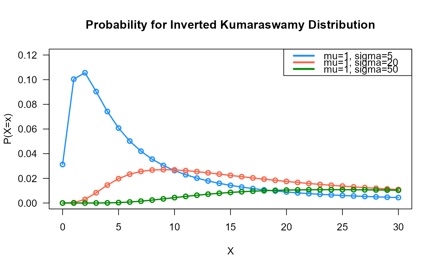
# Example 1
# Plotting the mass function for different parameter values
x_max <- 30
probs1 <- dDIKUM(x=0:x_max, mu=1, sigma=5)
probs2 <- dDIKUM(x=0:x_max, mu=1, sigma=20)
probs3 <- dDIKUM(x=0:x_max, mu=1, sigma=50)
# To plot the first k values
plot(x=0:x_max, y=probs1, type="o", lwd=2, col="dodgerblue", las=1,
ylab="P(X=x)", xlab="X", main="Probability for Inverted Kumaraswamy Distribution",
ylim=c(0, 0.12))
points(x=0:x_max, y=probs2, type="o", lwd=2, col="tomato")
points(x=0:x_max, y=probs3, type="o", lwd=2, col="green4")
legend("topright", col=c("dodgerblue", "tomato", "green4"), lwd=3,
legend=c("mu=1, sigma=5",
"mu=1, sigma=20",
"mu=1, sigma=50"))
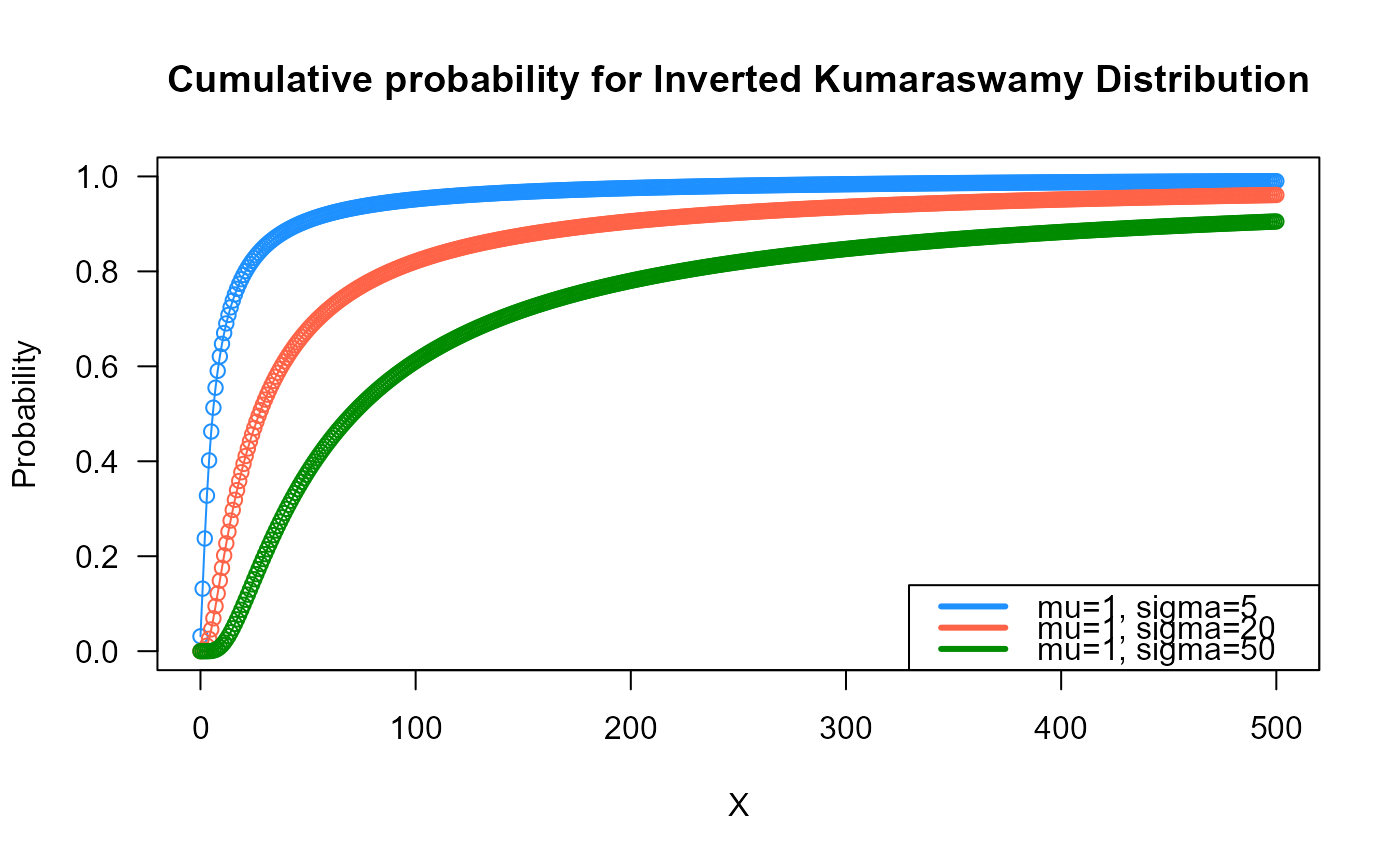
 # Example 2
# Checking if the cumulative curves converge to 1
x_max <- 500
cumulative_probs1 <- pDIKUM(q=0:x_max, mu=1, sigma=5)
cumulative_probs2 <- pDIKUM(q=0:x_max, mu=1, sigma=20)
cumulative_probs3 <- pDIKUM(q=0:x_max, mu=1, sigma=50)
plot(x=0:x_max, y=cumulative_probs1, col="dodgerblue",
type="o", las=1, ylim=c(0, 1),
main="Cumulative probability for Inverted Kumaraswamy Distribution",
xlab="X", ylab="Probability")
points(x=0:x_max, y=cumulative_probs2, type="o", col="tomato")
points(x=0:x_max, y=cumulative_probs3, type="o", col="green4")
legend("bottomright", col=c("dodgerblue", "tomato", "green4"), lwd=3,
legend=c("mu=1, sigma=5",
"mu=1, sigma=20",
"mu=1, sigma=50"))
# Example 2
# Checking if the cumulative curves converge to 1
x_max <- 500
cumulative_probs1 <- pDIKUM(q=0:x_max, mu=1, sigma=5)
cumulative_probs2 <- pDIKUM(q=0:x_max, mu=1, sigma=20)
cumulative_probs3 <- pDIKUM(q=0:x_max, mu=1, sigma=50)
plot(x=0:x_max, y=cumulative_probs1, col="dodgerblue",
type="o", las=1, ylim=c(0, 1),
main="Cumulative probability for Inverted Kumaraswamy Distribution",
xlab="X", ylab="Probability")
points(x=0:x_max, y=cumulative_probs2, type="o", col="tomato")
points(x=0:x_max, y=cumulative_probs3, type="o", col="green4")
legend("bottomright", col=c("dodgerblue", "tomato", "green4"), lwd=3,
legend=c("mu=1, sigma=5",
"mu=1, sigma=20",
"mu=1, sigma=50"))
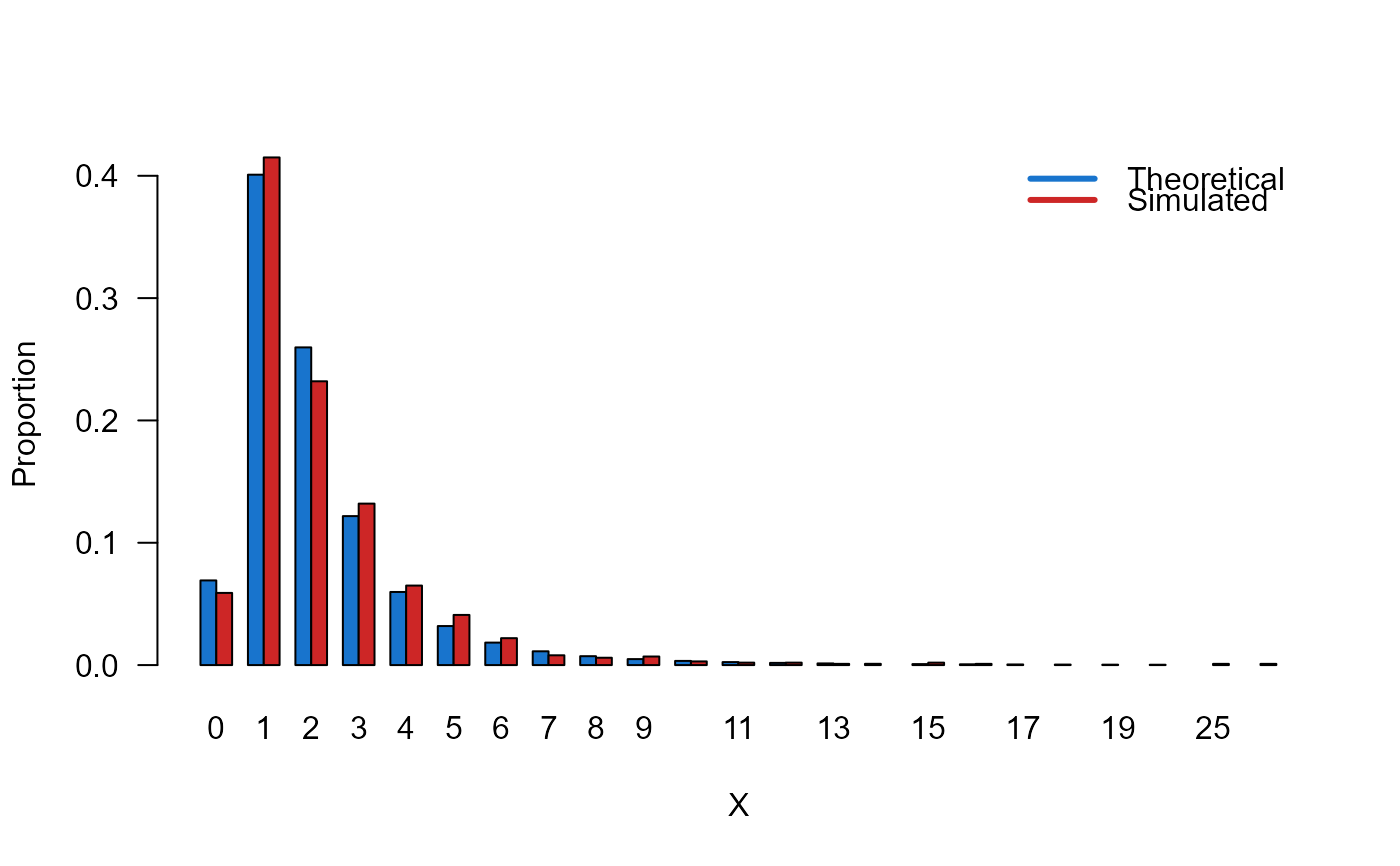
 # Example 3
# Comparing the random generator output with
# the theoretical probabilities
x_max <- 20
probs1 <- dDIKUM(x=0:x_max, mu=3, sigma=20)
names(probs1) <- 0:x_max
x <- rDIKUM(n=1000, mu=3, sigma=20)
probs2 <- prop.table(table(x))
cn <- union(names(probs1), names(probs2))
height <- rbind(probs1[cn], probs2[cn])
nombres <- cn
mp <- barplot(height, beside = TRUE, names.arg = nombres,
col=c("dodgerblue3","firebrick3"), las=1,
xlab="X", ylab="Proportion")
legend("topright",
legend=c("Theoretical", "Simulated"),
bty="n", lwd=3,
col=c("dodgerblue3","firebrick3"), lty=1)
# Example 3
# Comparing the random generator output with
# the theoretical probabilities
x_max <- 20
probs1 <- dDIKUM(x=0:x_max, mu=3, sigma=20)
names(probs1) <- 0:x_max
x <- rDIKUM(n=1000, mu=3, sigma=20)
probs2 <- prop.table(table(x))
cn <- union(names(probs1), names(probs2))
height <- rbind(probs1[cn], probs2[cn])
nombres <- cn
mp <- barplot(height, beside = TRUE, names.arg = nombres,
col=c("dodgerblue3","firebrick3"), las=1,
xlab="X", ylab="Proportion")
legend("topright",
legend=c("Theoretical", "Simulated"),
bty="n", lwd=3,
col=c("dodgerblue3","firebrick3"), lty=1)
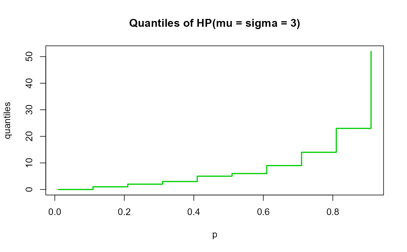
 # Example 4
# Checking the quantile function
mu <- 1
sigma <- 5
p <- seq(from=0.01, to=0.99, by=0.1)
qxx <- qDIKUM(p=p, mu=mu, sigma=sigma, lower.tail=TRUE, log.p=FALSE)
plot(p, qxx, type="s", lwd=2, col="green3", ylab="quantiles",
main="Quantiles of HP(mu = sigma = 3)")
# Example 4
# Checking the quantile function
mu <- 1
sigma <- 5
p <- seq(from=0.01, to=0.99, by=0.1)
qxx <- qDIKUM(p=p, mu=mu, sigma=sigma, lower.tail=TRUE, log.p=FALSE)
plot(p, qxx, type="s", lwd=2, col="green3", ylab="quantiles",
main="Quantiles of HP(mu = sigma = 3)")