These functions define the density, distribution function, quantile function and random generation for the Comway-Maxwell-Poisson distribution with parameters \(\mu\) and \(\sigma\). This parameterization was proposed by Ribeiro et al. (2020) and the main characteristic is that \(E(X)=\mu\).
dCOMPO2(x, mu, sigma, log = FALSE)

pCOMPO2(q, mu, sigma, lower.tail = TRUE, log.p = FALSE)

qCOMPO2(p, mu, sigma, lower.tail = TRUE, log.p = FALSE)

rCOMPO2(n, mu, sigma)
Arguments
- x, q
vector of (non-negative integer) quantiles.
- mu
vector of the mu parameter.
- sigma
vector of the sigma parameter.
- log, log.p
logical; if TRUE, probabilities p are given as log(p).
- lower.tail
logical; if TRUE (default), probabilities are \(P[X <= x]\), otherwise, \(P[X > x]\).
- p
vector of probabilities.
- n
number of random values to return.
Value
dCOMPO2 gives the density, pCOMPO2 gives the distribution
function, qCOMPO2 gives the quantile function, rCOMPO2
generates random deviates.
Details
The COMPO2 distribution with parameters \(\mu\) and \(\sigma\) has a support 0, 1, 2, ... and mass function given by
\(f(x | \mu, \sigma) = \left(\mu + \frac{\exp(\sigma)-1}{2 \exp(\sigma)} \right)^{x \exp(\sigma)} \frac{(x!)^{\exp(\sigma)}}{Z(\mu, \sigma)} \)
with \(\mu > 0\), \(\sigma \in \Re\) and
\(Z(\mu, \sigma)=\sum_{j=0}^{\infty} \frac{\mu^j}{(j!)^\sigma}\).
The proposed functions here are based on the functions from the COMPoissonReg package.
References
Ribeiro Jr, Eduardo E., et al. "Reparametrization of COM–Poisson regression models with applications in the analysis of experimental data." Statistical Modelling 20.5 (2020): 443-466.
See also
Examples
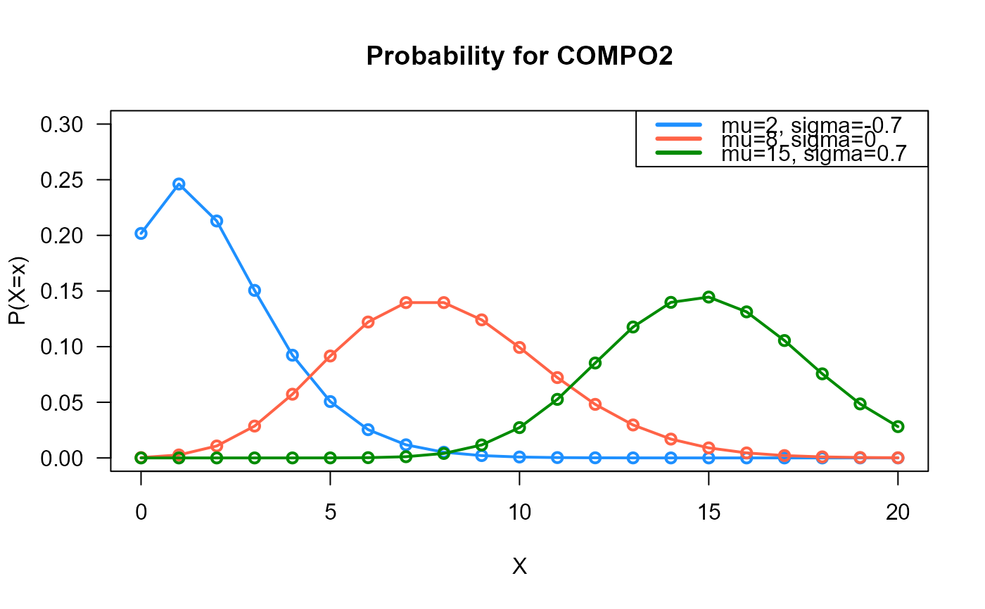
# Example 1
# Plotting the mass function for different parameter values
x_max <- 20
probs1 <- dCOMPO2(x=0:x_max, mu=2, sigma=-0.7)
probs2 <- dCOMPO2(x=0:x_max, mu=8, sigma=0)
probs3 <- dCOMPO2(x=0:x_max, mu=15, sigma=0.7)
# To plot the first k values
plot(x=0:x_max, y=probs1, type="o", lwd=2, col="dodgerblue", las=1,
ylab="P(X=x)", xlab="X", main="Probability for COMPO2",
ylim=c(0, 0.30))
points(x=0:x_max, y=probs2, type="o", lwd=2, col="tomato")
points(x=0:x_max, y=probs3, type="o", lwd=2, col="green4")
legend("topright", col=c("dodgerblue", "tomato", "green4"), lwd=3,
legend=c("mu=2, sigma=-0.7",
"mu=8, sigma=0",
"mu=15, sigma=0.7"))
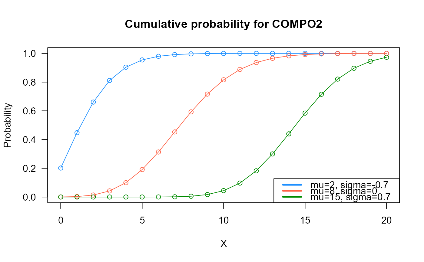
 # Example 2
# Checking if the cumulative curves converge to 1
x_max <- 20
cumulative_probs1 <- pCOMPO2(q=0:x_max, mu=2, sigma=-0.7)
cumulative_probs2 <- pCOMPO2(q=0:x_max, mu=8, sigma=0)
cumulative_probs3 <- pCOMPO2(q=0:x_max, mu=15, sigma=0.7)
plot(x=0:x_max, y=cumulative_probs1, col="dodgerblue",
type="o", las=1, ylim=c(0, 1),
main="Cumulative probability for COMPO2",
xlab="X", ylab="Probability")
points(x=0:x_max, y=cumulative_probs2, type="o", col="tomato")
points(x=0:x_max, y=cumulative_probs3, type="o", col="green4")
legend("bottomright", col=c("dodgerblue", "tomato", "green4"), lwd=3,
legend=c("mu=2, sigma=-0.7",
"mu=8, sigma=0",
"mu=15, sigma=0.7"))
# Example 2
# Checking if the cumulative curves converge to 1
x_max <- 20
cumulative_probs1 <- pCOMPO2(q=0:x_max, mu=2, sigma=-0.7)
cumulative_probs2 <- pCOMPO2(q=0:x_max, mu=8, sigma=0)
cumulative_probs3 <- pCOMPO2(q=0:x_max, mu=15, sigma=0.7)
plot(x=0:x_max, y=cumulative_probs1, col="dodgerblue",
type="o", las=1, ylim=c(0, 1),
main="Cumulative probability for COMPO2",
xlab="X", ylab="Probability")
points(x=0:x_max, y=cumulative_probs2, type="o", col="tomato")
points(x=0:x_max, y=cumulative_probs3, type="o", col="green4")
legend("bottomright", col=c("dodgerblue", "tomato", "green4"), lwd=3,
legend=c("mu=2, sigma=-0.7",
"mu=8, sigma=0",
"mu=15, sigma=0.7"))
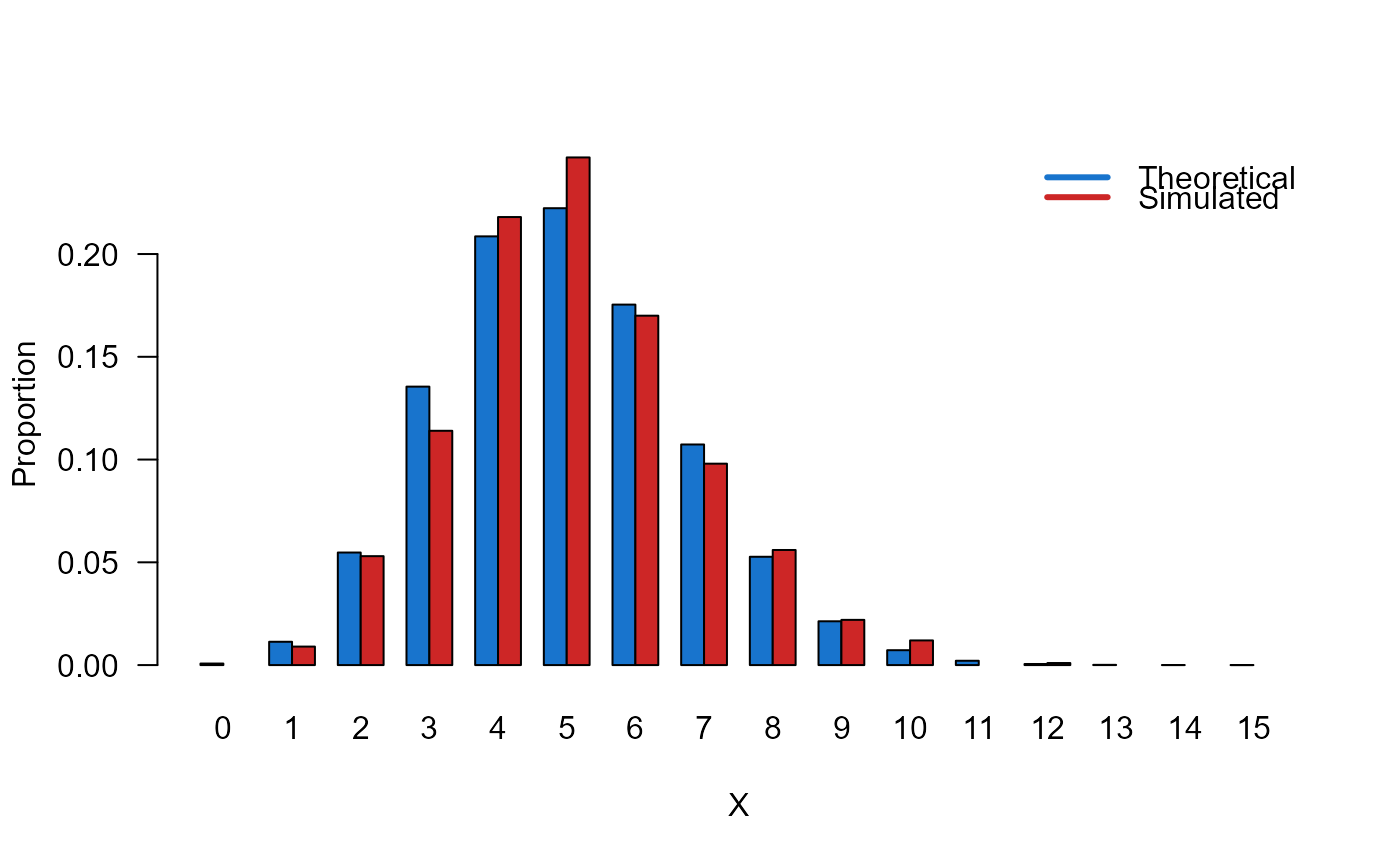
 # Example 3
# Comparing the random generator output with
# the theoretical probabilities
x_max <- 15
probs1 <- dCOMPO2(x=0:x_max, mu=5, sigma=0.5)
names(probs1) <- 0:x_max
x <- rCOMPO2(n=1000, mu=5, sigma=0.5)
probs2 <- prop.table(table(x))
cn <- union(names(probs1), names(probs2))
height <- rbind(probs1[cn], probs2[cn])
mp <- barplot(height, beside = TRUE, names.arg = cn,
col=c("dodgerblue3","firebrick3"), las=1,
xlab="X", ylab="Proportion")
legend("topright",
legend=c("Theoretical", "Simulated"),
bty="n", lwd=3,
col=c("dodgerblue3","firebrick3"), lty=1)
# Example 3
# Comparing the random generator output with
# the theoretical probabilities
x_max <- 15
probs1 <- dCOMPO2(x=0:x_max, mu=5, sigma=0.5)
names(probs1) <- 0:x_max
x <- rCOMPO2(n=1000, mu=5, sigma=0.5)
probs2 <- prop.table(table(x))
cn <- union(names(probs1), names(probs2))
height <- rbind(probs1[cn], probs2[cn])
mp <- barplot(height, beside = TRUE, names.arg = cn,
col=c("dodgerblue3","firebrick3"), las=1,
xlab="X", ylab="Proportion")
legend("topright",
legend=c("Theoretical", "Simulated"),
bty="n", lwd=3,
col=c("dodgerblue3","firebrick3"), lty=1)
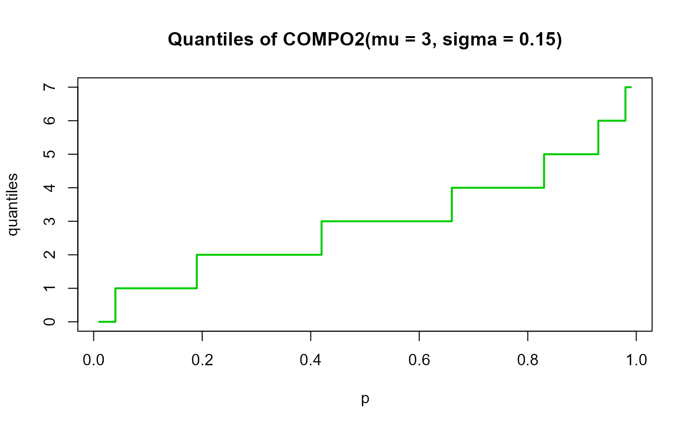
 # Example 4
# Checking the quantile function
mu <- 3
sigma <- 0.15
p <- seq(from=0.01, to=0.99, by=0.01)
qxx <- qCOMPO2(p=p, mu=mu, sigma=sigma, lower.tail=TRUE, log.p=FALSE)
plot(p, qxx, type="s", lwd=2, col="green3", ylab="quantiles",
main="Quantiles of COMPO2(mu = 3, sigma = 0.15)")
# Example 4
# Checking the quantile function
mu <- 3
sigma <- 0.15
p <- seq(from=0.01, to=0.99, by=0.01)
qxx <- qCOMPO2(p=p, mu=mu, sigma=sigma, lower.tail=TRUE, log.p=FALSE)
plot(p, qxx, type="s", lwd=2, col="green3", ylab="quantiles",
main="Quantiles of COMPO2(mu = 3, sigma = 0.15)")