These functions define the density, distribution function, quantile function and random generation for the Conway-Maxwell-Poisson distribution with parameters \(\mu\) and \(\sigma\).
dCOMPO(x, mu, sigma, log = FALSE)

pCOMPO(q, mu, sigma, lower.tail = TRUE, log.p = FALSE)

qCOMPO(p, mu, sigma, lower.tail = TRUE, log.p = FALSE)

rCOMPO(n, mu, sigma)
Arguments
- x, q
vector of (non-negative integer) quantiles.
- mu
vector of the mu parameter.
- sigma
vector of the sigma parameter.
- log, log.p
logical; if TRUE, probabilities p are given as log(p).
- lower.tail
logical; if TRUE (default), probabilities are \(P[X <= x]\), otherwise, \(P[X > x]\).
- p
vector of probabilities.
- n
number of random values to return.
Value
dCOMPO gives the density, pCOMPO gives the distribution
function, qCOMPO gives the quantile function, rCOMPO
generates random deviates.
Details
The COMPO distribution with parameters \(\mu\) and \(\sigma\) has a support 0, 1, 2, ... and mass function given by
\(f(x | \mu, \sigma) = \frac{\mu^x}{(x!)^{\sigma} Z(\mu, \sigma)} \)
with \(\mu > 0\), \(\sigma \geq 0\) and
\(Z(\mu, \sigma)=\sum_{j=0}^{\infty} \frac{\mu^j}{(j!)^\sigma}\).
The proposed functions here are based on the functions from the COMPoissonReg package.
References
Shmueli, G., Minka, T. P., Kadane, J. B., Borle, S., & Boatwright, P. (2005). A useful distribution for fitting discrete data: revival of the Conway–Maxwell–Poisson distribution. Journal of the Royal Statistical Society Series C: Applied Statistics, 54(1), 127-142.
See also
Examples
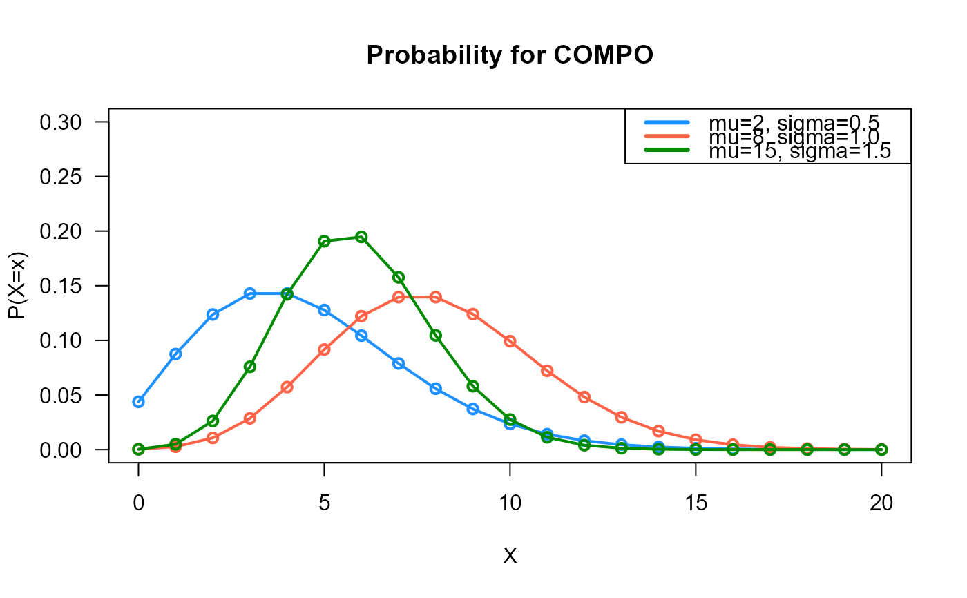
# Example 1
# Plotting the mass function for different parameter values
x_max <- 20
probs1 <- dCOMPO(x=0:x_max, mu=2, sigma=0.5)
probs2 <- dCOMPO(x=0:x_max, mu=8, sigma=1.0)
probs3 <- dCOMPO(x=0:x_max, mu=15, sigma=1.5)
# To plot the first k values
plot(x=0:x_max, y=probs1, type="o", lwd=2, col="dodgerblue", las=1,
ylab="P(X=x)", xlab="X", main="Probability for COMPO",
ylim=c(0, 0.30))
points(x=0:x_max, y=probs2, type="o", lwd=2, col="tomato")
points(x=0:x_max, y=probs3, type="o", lwd=2, col="green4")
legend("topright", col=c("dodgerblue", "tomato", "green4"), lwd=3,
legend=c("mu=2, sigma=0.5",
"mu=8, sigma=1.0",
"mu=15, sigma=1.5"))
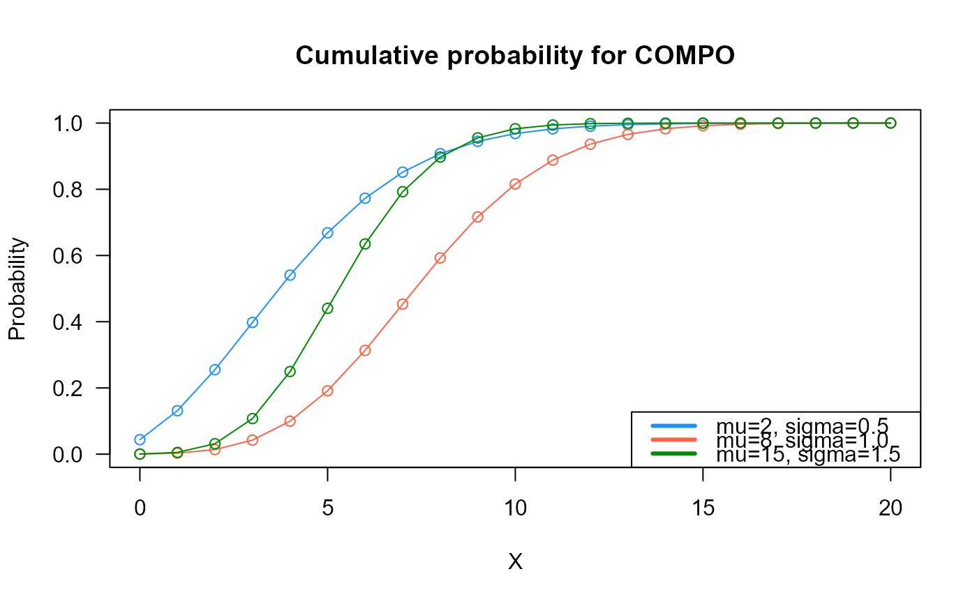
 # Example 2
# Checking if the cumulative curves converge to 1
x_max <- 20
cumulative_probs1 <- pCOMPO(q=0:x_max, mu=2, sigma=0.5)
cumulative_probs2 <- pCOMPO(q=0:x_max, mu=8, sigma=1.0)
cumulative_probs3 <- pCOMPO(q=0:x_max, mu=15, sigma=1.5)
plot(x=0:x_max, y=cumulative_probs1, col="dodgerblue",
type="o", las=1, ylim=c(0, 1),
main="Cumulative probability for COMPO",
xlab="X", ylab="Probability")
points(x=0:x_max, y=cumulative_probs2, type="o", col="tomato")
points(x=0:x_max, y=cumulative_probs3, type="o", col="green4")
legend("bottomright", col=c("dodgerblue", "tomato", "green4"), lwd=3,
legend=c("mu=2, sigma=0.5",
"mu=8, sigma=1.0",
"mu=15, sigma=1.5"))
# Example 2
# Checking if the cumulative curves converge to 1
x_max <- 20
cumulative_probs1 <- pCOMPO(q=0:x_max, mu=2, sigma=0.5)
cumulative_probs2 <- pCOMPO(q=0:x_max, mu=8, sigma=1.0)
cumulative_probs3 <- pCOMPO(q=0:x_max, mu=15, sigma=1.5)
plot(x=0:x_max, y=cumulative_probs1, col="dodgerblue",
type="o", las=1, ylim=c(0, 1),
main="Cumulative probability for COMPO",
xlab="X", ylab="Probability")
points(x=0:x_max, y=cumulative_probs2, type="o", col="tomato")
points(x=0:x_max, y=cumulative_probs3, type="o", col="green4")
legend("bottomright", col=c("dodgerblue", "tomato", "green4"), lwd=3,
legend=c("mu=2, sigma=0.5",
"mu=8, sigma=1.0",
"mu=15, sigma=1.5"))
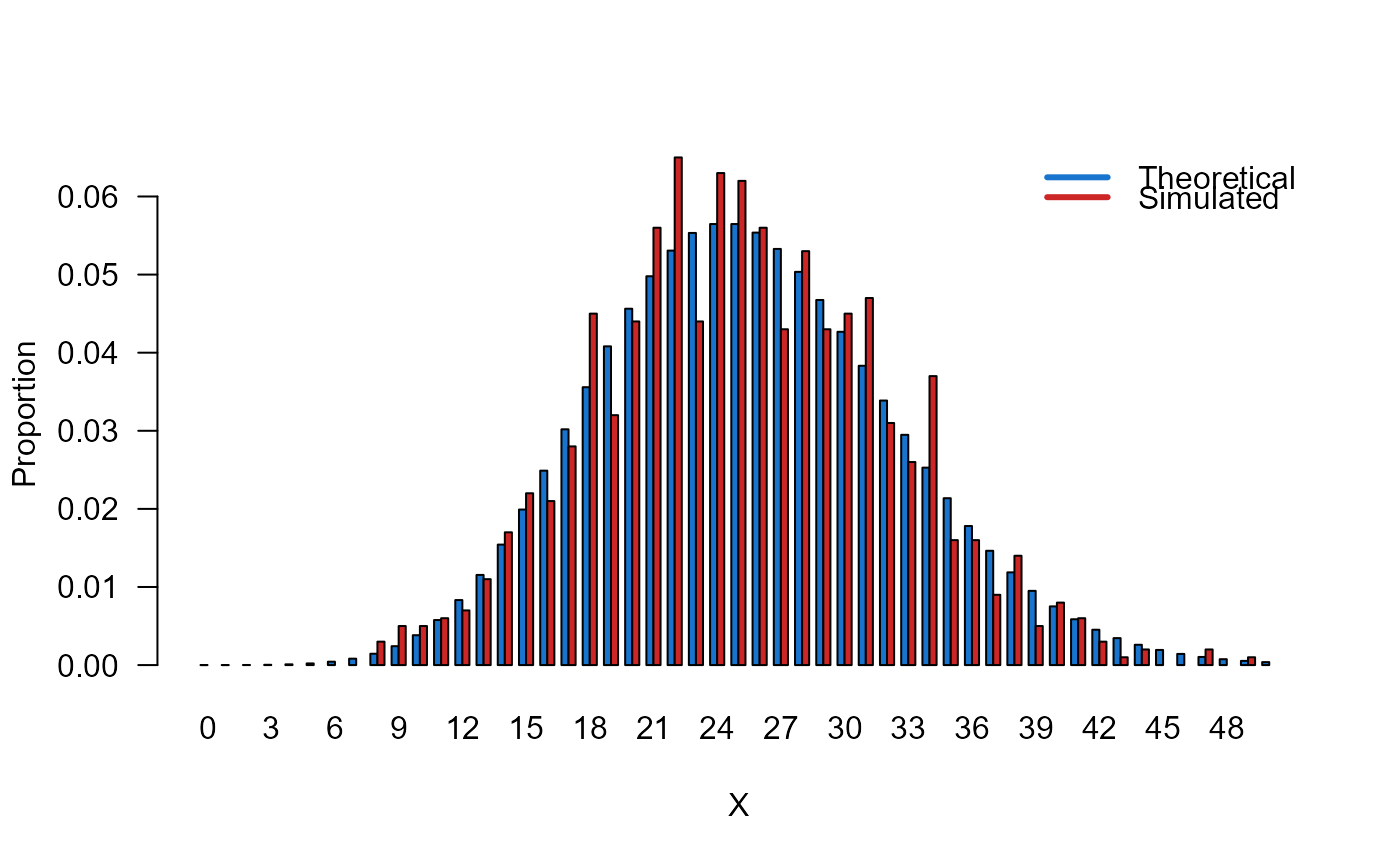
 # Example 3
# Comparing the random generator output with
# the theoretical probabilities
x_max <- 50
probs1 <- dCOMPO(x=0:x_max, mu=5, sigma=0.5)
names(probs1) <- 0:x_max
x <- rCOMPO(n=1000, mu=5, sigma=0.5)
probs2 <- prop.table(table(x))
cn <- union(names(probs1), names(probs2))
height <- rbind(probs1[cn], probs2[cn])
mp <- barplot(height, beside = TRUE, names.arg = cn,
col=c("dodgerblue3","firebrick3"), las=1,
xlab="X", ylab="Proportion")
legend("topright",
legend=c("Theoretical", "Simulated"),
bty="n", lwd=3,
col=c("dodgerblue3","firebrick3"), lty=1)
# Example 3
# Comparing the random generator output with
# the theoretical probabilities
x_max <- 50
probs1 <- dCOMPO(x=0:x_max, mu=5, sigma=0.5)
names(probs1) <- 0:x_max
x <- rCOMPO(n=1000, mu=5, sigma=0.5)
probs2 <- prop.table(table(x))
cn <- union(names(probs1), names(probs2))
height <- rbind(probs1[cn], probs2[cn])
mp <- barplot(height, beside = TRUE, names.arg = cn,
col=c("dodgerblue3","firebrick3"), las=1,
xlab="X", ylab="Proportion")
legend("topright",
legend=c("Theoretical", "Simulated"),
bty="n", lwd=3,
col=c("dodgerblue3","firebrick3"), lty=1)
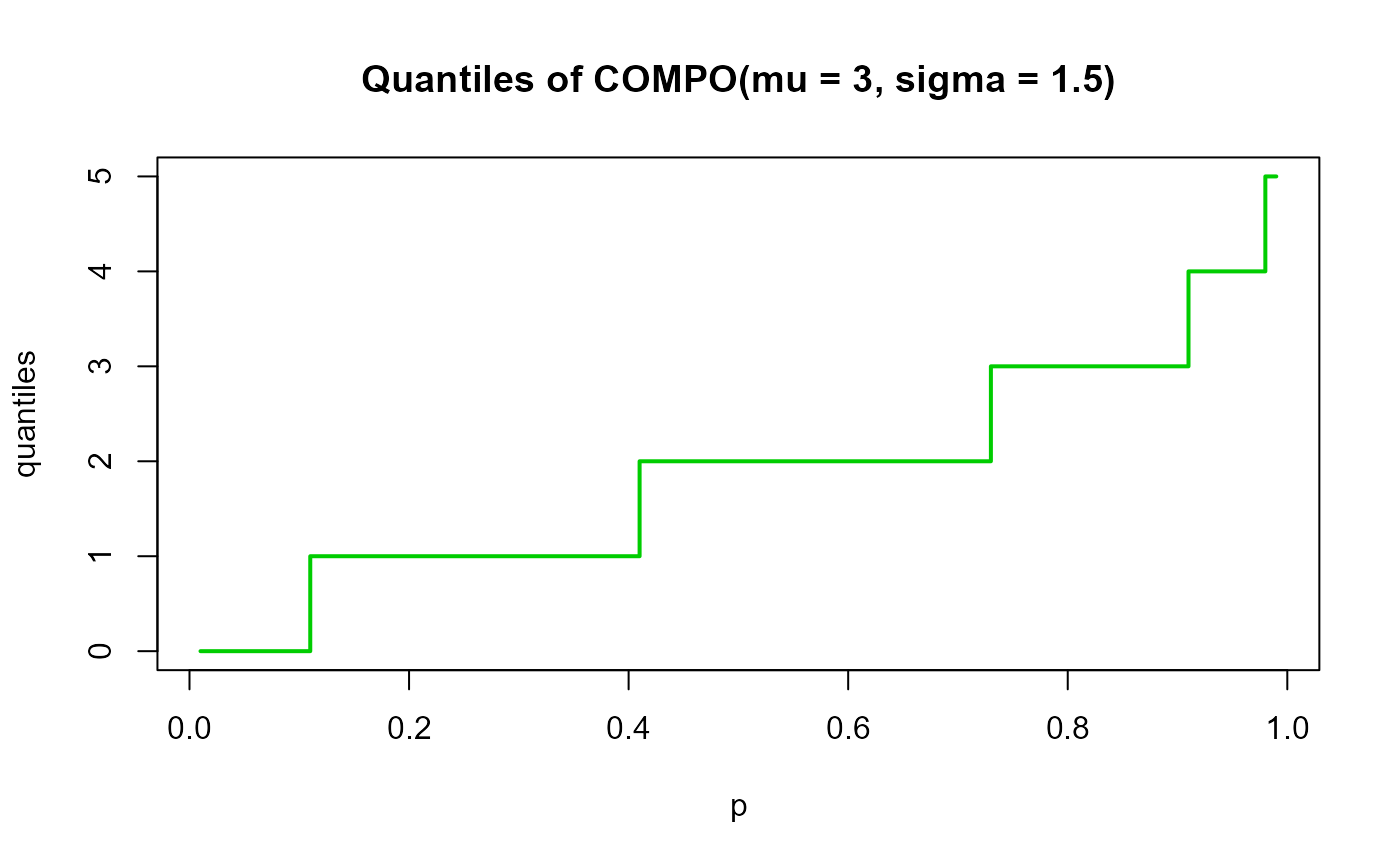
 # Example 4
# Checking the quantile function
mu <- 3
sigma <- 1.5
p <- seq(from=0.01, to=0.99, by=0.01)
qxx <- qCOMPO(p=p, mu=mu, sigma=sigma, lower.tail=TRUE, log.p=FALSE)
plot(p, qxx, type="s", lwd=2, col="green3", ylab="quantiles",
main="Quantiles of COMPO(mu = 3, sigma = 1.5)")
# Example 4
# Checking the quantile function
mu <- 3
sigma <- 1.5
p <- seq(from=0.01, to=0.99, by=0.01)
qxx <- qCOMPO(p=p, mu=mu, sigma=sigma, lower.tail=TRUE, log.p=FALSE)
plot(p, qxx, type="s", lwd=2, col="green3", ylab="quantiles",
main="Quantiles of COMPO(mu = 3, sigma = 1.5)")