These functions define the density, distribution function, quantile function and random generation for the Unit Half Logistic-Geometry distribution with parameter \(\mu\).
dUHLG(x, mu, log = FALSE)

pUHLG(q, mu, lower.tail = TRUE, log.p = FALSE)

qUHLG(p, mu, lower.tail = TRUE, log.p = FALSE)

rUHLG(n, mu)
Arguments
- x, q
vector of (non-negative integer) quantiles.
- mu
vector of the mu parameter.
- log, log.p
logical; if TRUE, probabilities p are given as log(p).
- lower.tail
logical; if TRUE (default), probabilities are \(P[X <= x]\), otherwise, \(P[X > x]\).
- p
vector of probabilities.
- n
number of random values to return.
Value
dUHLG gives the density, pUHLG gives the distribution
function, qUHLG gives the quantile function, rUHLG
generates random deviates.
Details
The Unit Half Logistic-Geometry distribution with parameter \(\mu\) has a support in \((0, 1)\) and density given by
\(f(x| \mu) = \frac{2 \mu}{(\mu+(2-\mu)x)^2} \)
for \(0 < x < 1\) and \(\mu > 0\).
References
Ramadan, A. T., Tolba, A. H., & El-Desouky, B. S. (2022). A unit half-logistic geometric distribution and its application in insurance. Axioms, 11(12), 676.
See also
UHLG.
Examples
# Example 1
# Plotting the density function for different parameter values
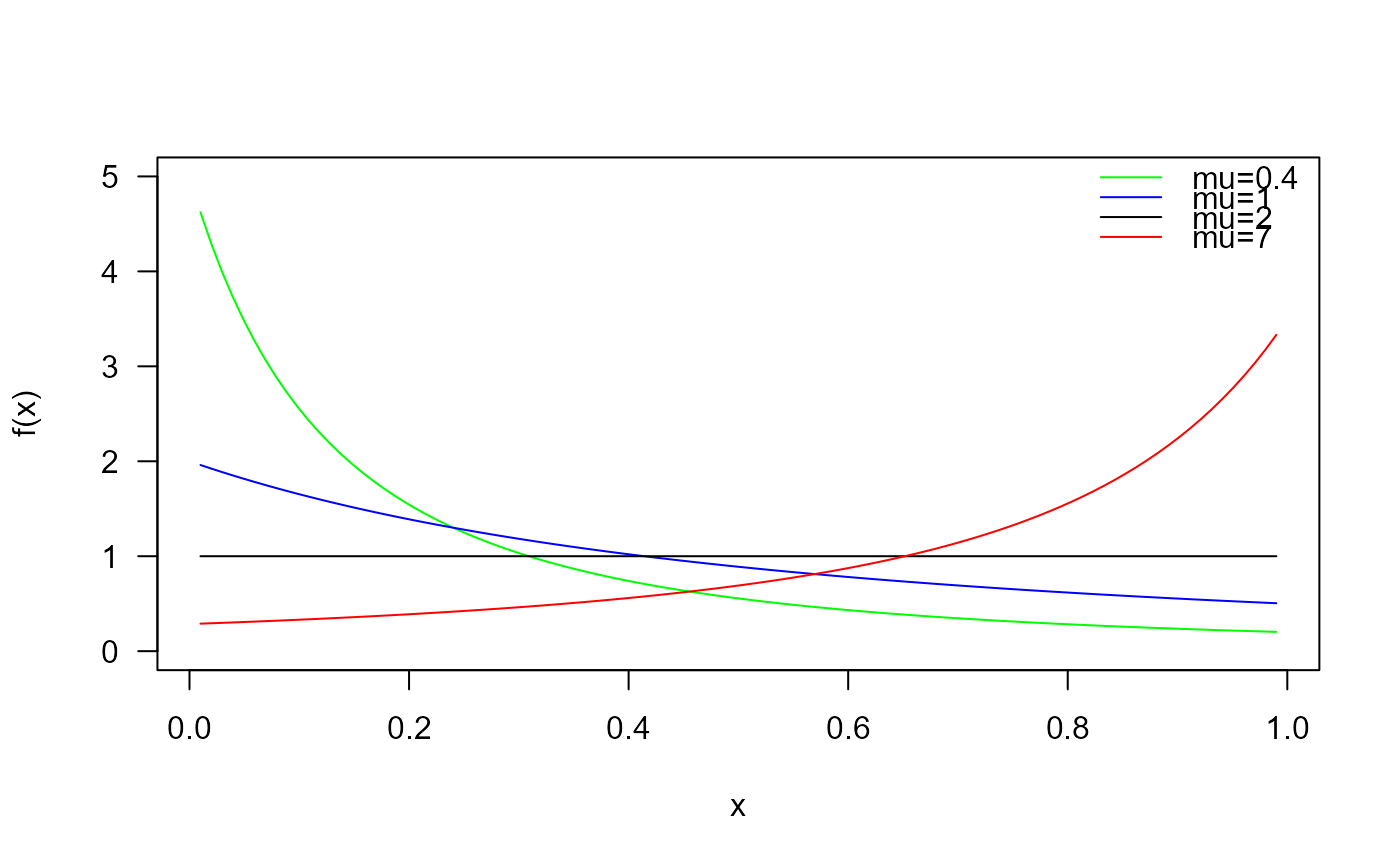
curve(dUHLG(x, mu=0.4), from=0.01, to=0.99,
ylim=c(0, 5), lwd=2,
col="black", las=1, ylab="f(x)")
curve(dUHLG(x, mu=1), lwd=2,
add=TRUE, col="red")
curve(dUHLG(x, mu=2), lwd=2,
add=TRUE, col="green")
curve(dUHLG(x, mu=7), lwd=2,
add=TRUE, col="blue")
legend("topright",
col=c("black", "red", "green", "blue"),
lty=1, bty="n", lwd=2,
legend=c("mu=0.4",
"mu=1",
"mu=2",
"mu=7"))
 # Example 2
# Checking if the cumulative curves converge to 1
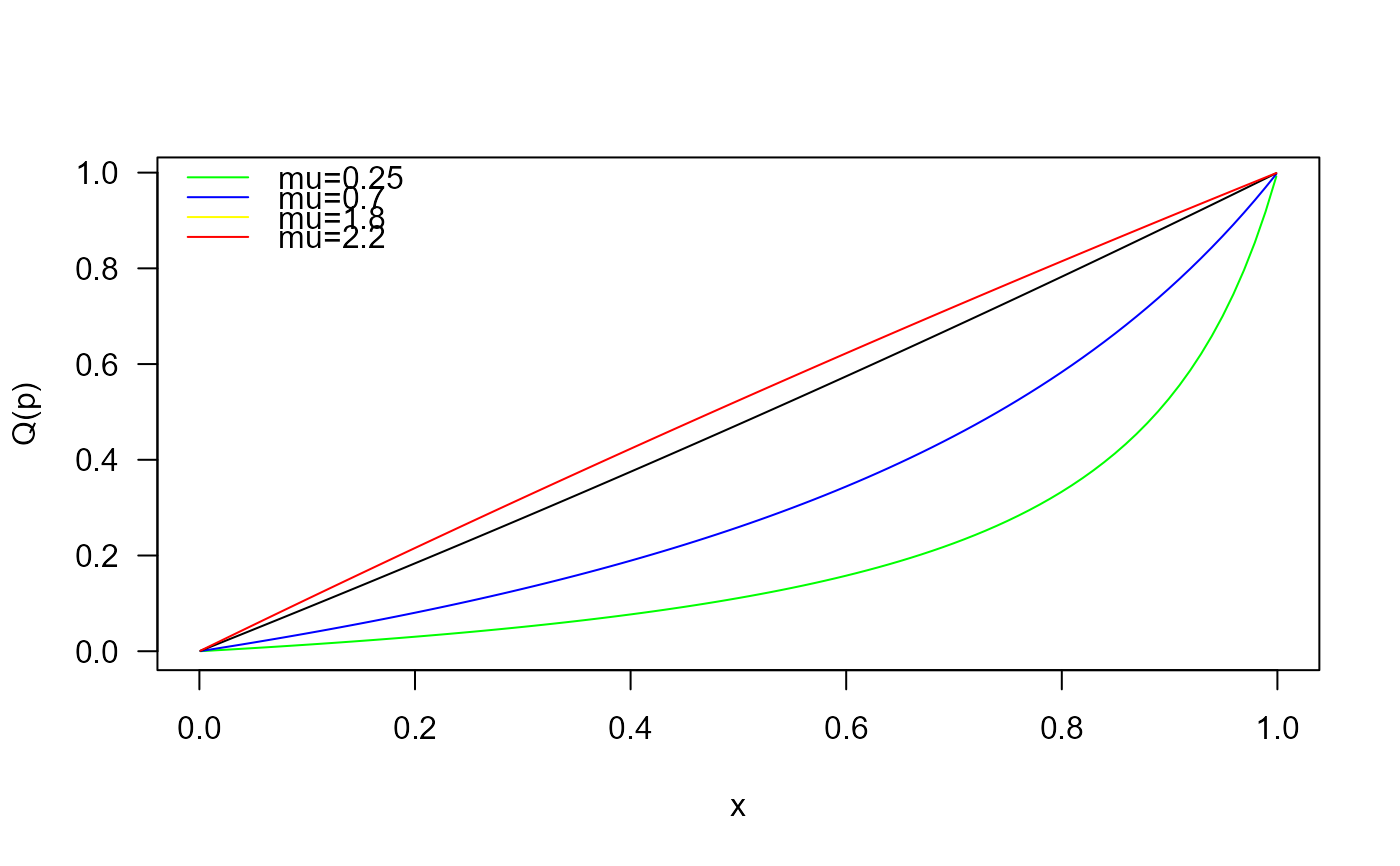
curve(pUHLG(x, mu=0.25), lwd=2,
from=0.001, to=0.999, col="black", las=1, ylab="F(x)")
curve(pUHLG(x, mu=0.7), lwd=2,
add=TRUE, col="red")
curve(pUHLG(x, mu=1.8), lwd=2,
add=TRUE, col="green")
curve(pUHLG(x, mu=2.2), lwd=2,
add=TRUE, col="blue")
legend("bottomright", col=c("black", "red", "green", "blue"),
lty=1, bty="n", lwd=2,
legend=c("mu=0.25",
"mu=0.7",
"mu=1.8",
"mu=2.2"))
# Example 2
# Checking if the cumulative curves converge to 1
curve(pUHLG(x, mu=0.25), lwd=2,
from=0.001, to=0.999, col="black", las=1, ylab="F(x)")
curve(pUHLG(x, mu=0.7), lwd=2,
add=TRUE, col="red")
curve(pUHLG(x, mu=1.8), lwd=2,
add=TRUE, col="green")
curve(pUHLG(x, mu=2.2), lwd=2,
add=TRUE, col="blue")
legend("bottomright", col=c("black", "red", "green", "blue"),
lty=1, bty="n", lwd=2,
legend=c("mu=0.25",
"mu=0.7",
"mu=1.8",
"mu=2.2"))
 # Example 3
# Checking the quantile function
mu <- 2
p <- seq(from=0.01, to=0.99, length.out=100)
plot(x=qUHLG(p, mu=mu), y=p,
xlab="Quantile", las=1, ylab="Probability")
curve(pUHLG(x, mu=mu), add=TRUE, col="red")
# Example 3
# Checking the quantile function
mu <- 2
p <- seq(from=0.01, to=0.99, length.out=100)
plot(x=qUHLG(p, mu=mu), y=p,
xlab="Quantile", las=1, ylab="Probability")
curve(pUHLG(x, mu=mu), add=TRUE, col="red")
 # Example 4
# Comparing the random generator output with
# the theoretical density
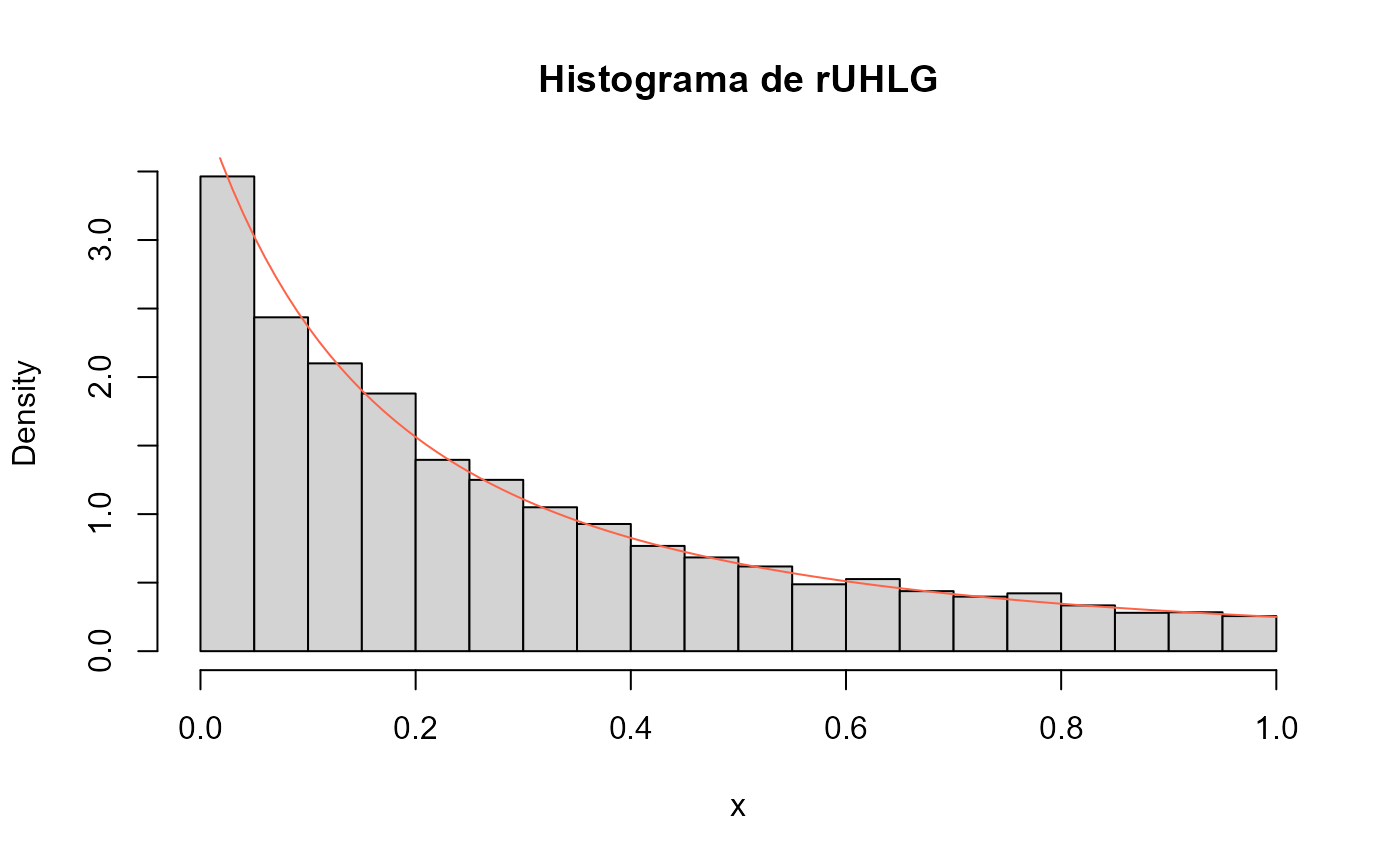
x <- rUHLG(n=10000, mu=0.5)
hist(x, freq=FALSE)
curve(dUHLG(x, mu=0.5), lwd=2,
col="tomato", add=TRUE, from=0.01, to=0.99)
# Example 4
# Comparing the random generator output with
# the theoretical density
x <- rUHLG(n=10000, mu=0.5)
hist(x, freq=FALSE)
curve(dUHLG(x, mu=0.5), lwd=2,
col="tomato", add=TRUE, from=0.01, to=0.99)