These functions define the density, distribution function, quantile function and random generation for the Beta Rectangular distribution with parameters \(\mu\), \(\sigma\) and \(\nu\) reparameterized to ensure \(E(X)=\mu\).
dBER2(x, mu, sigma, nu, log = FALSE)

pBER2(q, mu, sigma, nu, lower.tail = TRUE, log.p = FALSE)

qBER2(p, mu, sigma, nu, lower.tail = TRUE, log.p = FALSE)

rBER2(n, mu, sigma, nu)
Arguments
- x, q
vector of (non-negative integer) quantiles.
- mu
vector of the mu parameter.
- sigma
vector of the sigma parameter.
- nu
vector of the nu parameter.
- log, log.p
logical; if TRUE, probabilities p are given as log(p).
- lower.tail
logical; if TRUE (default), probabilities are \(P[X <= x]\), otherwise, \(P[X > x]\).
- p
vector of probabilities.
- n
number of random values to return.
Details
The Beta Rectangular distribution with parameters \(\mu\), \(\sigma\) and \(\nu\) has a support in \((0, 1)\) and density given by
\(f(x| \mu, \sigma, \nu) = \nu + (1 - \nu) b(x| \mu, \sigma)\)
for \(0 < x < 1\), \(0 < \mu < 1\), \(\sigma > 0\) and \(0 < \nu < 1\).
The function \(b(.)\) corresponds to the traditional beta distribution
that can be computed by dbeta(x, shape1=mu*sigma, shape2=(1-mu)*sigma).
References
Bayes, C. L., Bazán, J. L., & García, C. (2012). A new robust regression model for proportions. Bayesian Analysis, 7(4), 841-866.
See also
BER2.
Examples
# Example 1
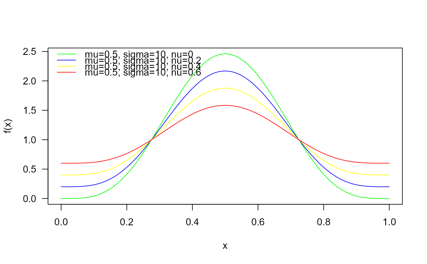
# Plotting the density function for different parameter values
curve(dBER2(x, mu=0.5, sigma=10, nu=0),
from=0, to=1, col="green", las=1, ylab="f(x)")
curve(dBER2(x, mu=0.5, sigma=10, nu=0.2),
add=TRUE, col= "blue1")
curve(dBER2(x, mu=0.5, sigma=10, nu=0.4),
add=TRUE, col="yellow")
curve(dBER2(x, mu=0.5, sigma=10, nu=0.6),
add=TRUE, col="red")
legend("topleft", col=c("green", "blue1", "yellow", "red"),
lty=1, bty="n",
legend=c("mu=0.5, sigma=10, nu=0",
"mu=0.5, sigma=10, nu=0.2",
"mu=0.5, sigma=10, nu=0.4",
"mu=0.5, sigma=10, nu=0.6"))
 curve(dBER2(x, mu=0.3, sigma=10, nu=0),
from=0, to=1, col="green", las=1, ylab="f(x)")
curve(dBER2(x, mu=0.3, sigma=10, nu=0.2),
add=TRUE, col= "blue1")
curve(dBER2(x, mu=0.3, sigma=10, nu=0.4),
add=TRUE, col="yellow")
curve(dBER2(x, mu=0.3, sigma=10, nu=0.6),
add=TRUE, col="red")
legend("topright", col=c("green", "blue1", "yellow", "red"),
lty=1, bty="n",
legend=c("mu=0.3, sigma=10, nu=0",
"mu=0.3, sigma=10, nu=0.2",
"mu=0.3, sigma=10, nu=0.4",
"mu=0.3, sigma=10, nu=0.6"))
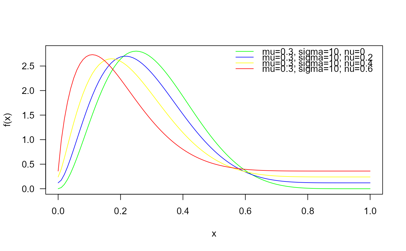
curve(dBER2(x, mu=0.3, sigma=10, nu=0),
from=0, to=1, col="green", las=1, ylab="f(x)")
curve(dBER2(x, mu=0.3, sigma=10, nu=0.2),
add=TRUE, col= "blue1")
curve(dBER2(x, mu=0.3, sigma=10, nu=0.4),
add=TRUE, col="yellow")
curve(dBER2(x, mu=0.3, sigma=10, nu=0.6),
add=TRUE, col="red")
legend("topright", col=c("green", "blue1", "yellow", "red"),
lty=1, bty="n",
legend=c("mu=0.3, sigma=10, nu=0",
"mu=0.3, sigma=10, nu=0.2",
"mu=0.3, sigma=10, nu=0.4",
"mu=0.3, sigma=10, nu=0.6"))
 # Example 2
# Checking if the cumulative curves converge to 1
curve(pBER2(x, mu=0.5, sigma=10, nu=0),
from=0, to=1, col="green", las=1, ylab="f(x)")
curve(pBER2(x, mu=0.5, sigma=10, nu=0.2),
add=TRUE, col= "blue1")
curve(pBER2(x, mu=0.5, sigma=10, nu=0.4),
add=TRUE, col="yellow")
curve(pBER2(x, mu=0.5, sigma=10, nu=0.6),
add=TRUE, col="red")
legend("topleft", col=c("green", "blue1", "yellow", "red"),
lty=1, bty="n",
legend=c("mu=0.5, sigma=10, nu=0",
"mu=0.5, sigma=10, nu=0.2",
"mu=0.5, sigma=10, nu=0.4",
"mu=0.5, sigma=10, nu=0.6"))
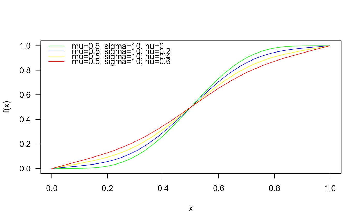
# Example 2
# Checking if the cumulative curves converge to 1
curve(pBER2(x, mu=0.5, sigma=10, nu=0),
from=0, to=1, col="green", las=1, ylab="f(x)")
curve(pBER2(x, mu=0.5, sigma=10, nu=0.2),
add=TRUE, col= "blue1")
curve(pBER2(x, mu=0.5, sigma=10, nu=0.4),
add=TRUE, col="yellow")
curve(pBER2(x, mu=0.5, sigma=10, nu=0.6),
add=TRUE, col="red")
legend("topleft", col=c("green", "blue1", "yellow", "red"),
lty=1, bty="n",
legend=c("mu=0.5, sigma=10, nu=0",
"mu=0.5, sigma=10, nu=0.2",
"mu=0.5, sigma=10, nu=0.4",
"mu=0.5, sigma=10, nu=0.6"))
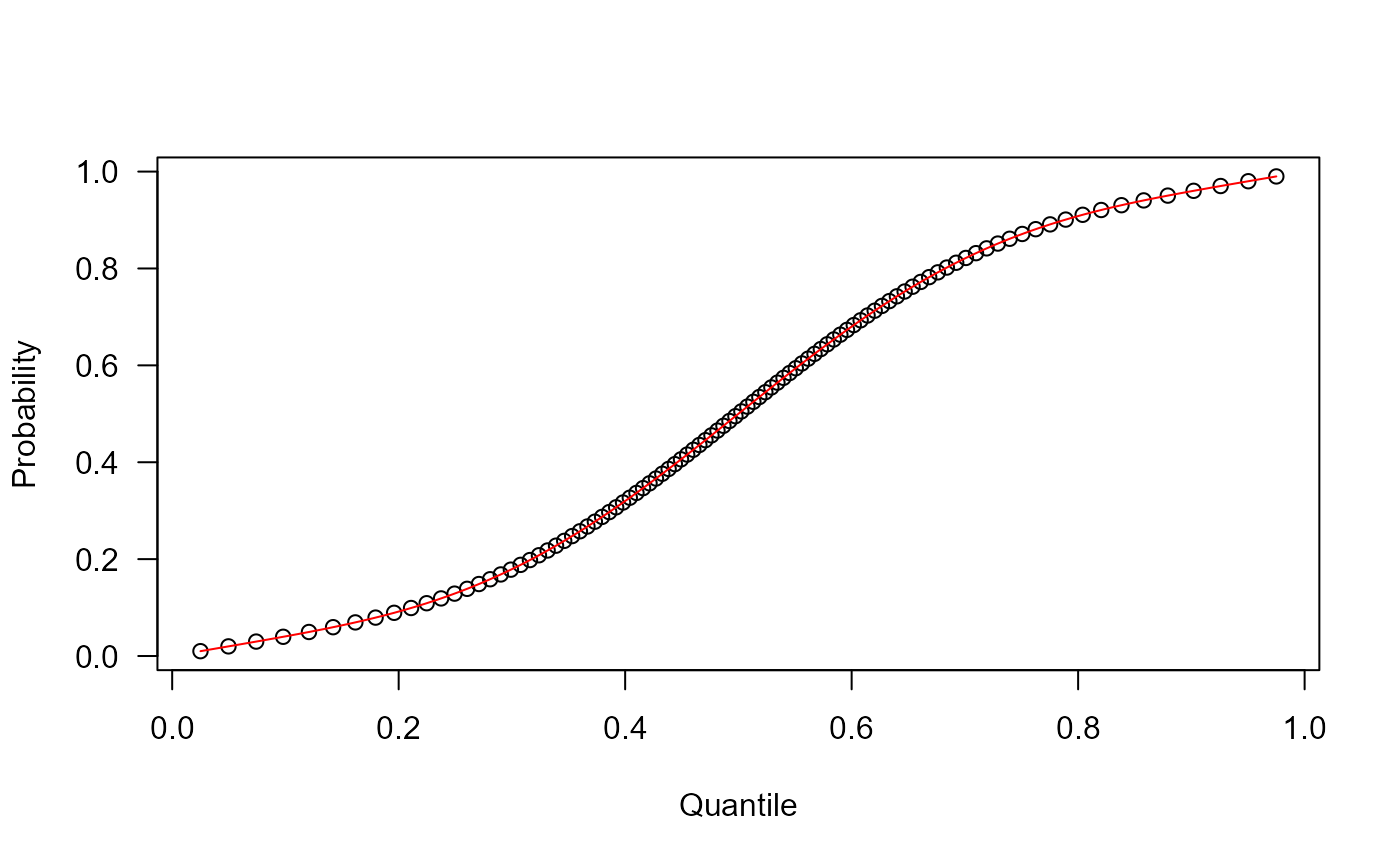
 # Example 3
# Checking the quantile function
mu <- 0.5
sigma <- 10
nu <- 0.4
p <- seq(from=0.01, to=0.99, length.out=100)
plot(x=qBER2(p, mu=mu, sigma=sigma, nu=nu), y=p,
xlab="Quantile", las=1, ylab="Probability")
curve(pBER2(x, mu=mu, sigma=sigma, nu=nu), add=TRUE, col="red")
# Example 3
# Checking the quantile function
mu <- 0.5
sigma <- 10
nu <- 0.4
p <- seq(from=0.01, to=0.99, length.out=100)
plot(x=qBER2(p, mu=mu, sigma=sigma, nu=nu), y=p,
xlab="Quantile", las=1, ylab="Probability")
curve(pBER2(x, mu=mu, sigma=sigma, nu=nu), add=TRUE, col="red")
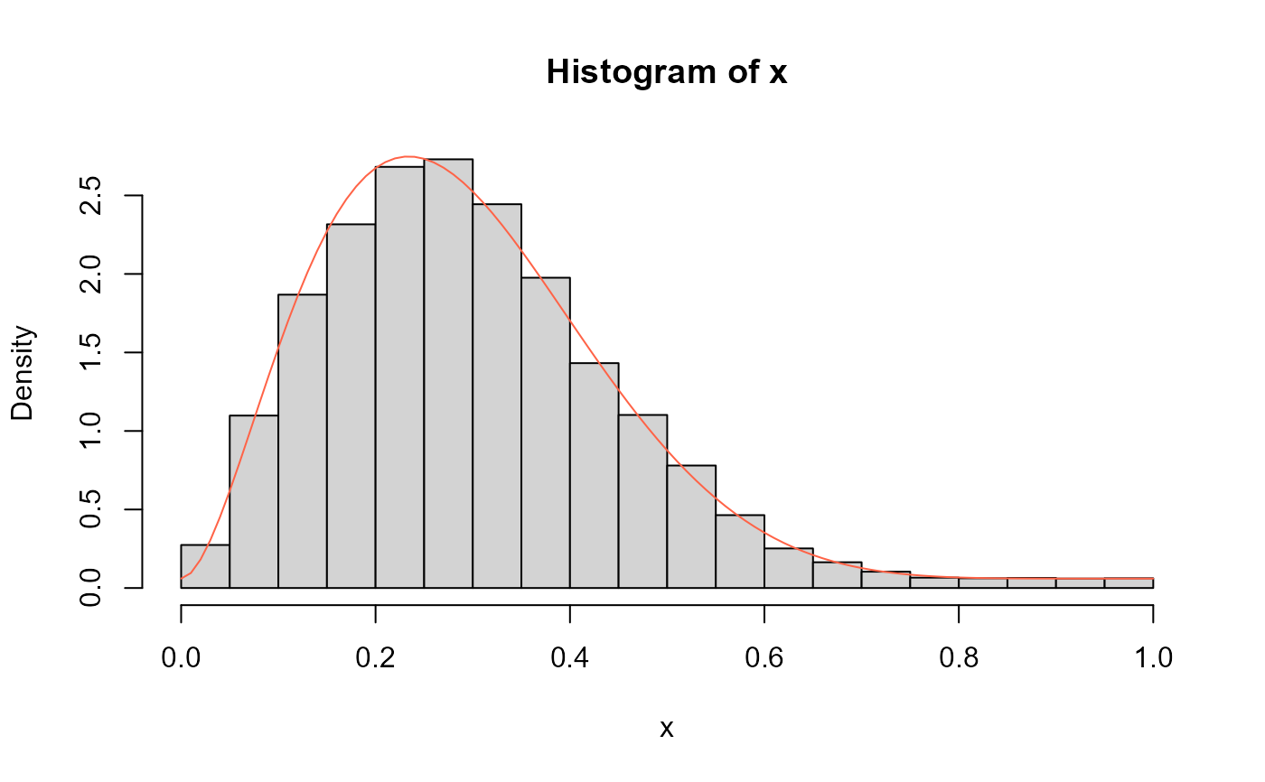
 # Example 4
# Comparing the random generator output with
# the theoretical density
x <- rBER2(n= 10000, mu=0.3, sigma=10, nu=0.1)
hist(x, freq=FALSE)
curve(dBER2(x, mu=0.3, sigma=10, nu=0.1),
col="tomato", add=TRUE)
# Example 4
# Comparing the random generator output with
# the theoretical density
x <- rBER2(n= 10000, mu=0.3, sigma=10, nu=0.1)
hist(x, freq=FALSE)
curve(dBER2(x, mu=0.3, sigma=10, nu=0.1),
col="tomato", add=TRUE)