These functions define the density, distribution function, quantile function and random generation for the Beta Rectangular distribution with parameters \(\mu\), \(\sigma\) and \(\nu\).
dBER(x, mu, sigma, nu, log = FALSE)

pBER(q, mu, sigma, nu, lower.tail = TRUE, log.p = FALSE)

qBER(p, mu, sigma, nu, lower.tail = TRUE, log.p = FALSE)

rBER(n, mu, sigma, nu)
Arguments
- x, q
vector of (non-negative integer) quantiles.
- mu
vector of the mu parameter.
- sigma
vector of the sigma parameter.
- nu
vector of the nu parameter.
- log, log.p
logical; if TRUE, probabilities p are given as log(p).
- lower.tail
logical; if TRUE (default), probabilities are \(P[X <= x]\), otherwise, \(P[X > x]\).
- p
vector of probabilities.
- n
number of random values to return.
Value
dBER gives the density, pBER gives the distribution
function, qBER gives the quantile function, rBER
generates random deviates.
Details
The Beta Rectangular distribution with parameters \(\mu\), \(\sigma\) and \(\nu\) has a support in \((0, 1)\) and density given by
\(f(x| \mu, \sigma, \nu) = \nu + (1 - \nu) b(x| \mu, \sigma)\)
for \(0 < x < 1\), \(0 < \mu < 1\), \(\sigma > 0\) and \(0 < \nu < 1\).
The function \(b(.)\) corresponds to the traditional beta distribution
that can be computed by dbeta(x, shape1=mu*sigma, shape2=(1-mu)*sigma).
References
Bayes, C. L., Bazán, J. L., & García, C. (2012). A new robust regression model for proportions. Bayesian Analysis, 7(4), 841-866.
See also
BER.
Examples
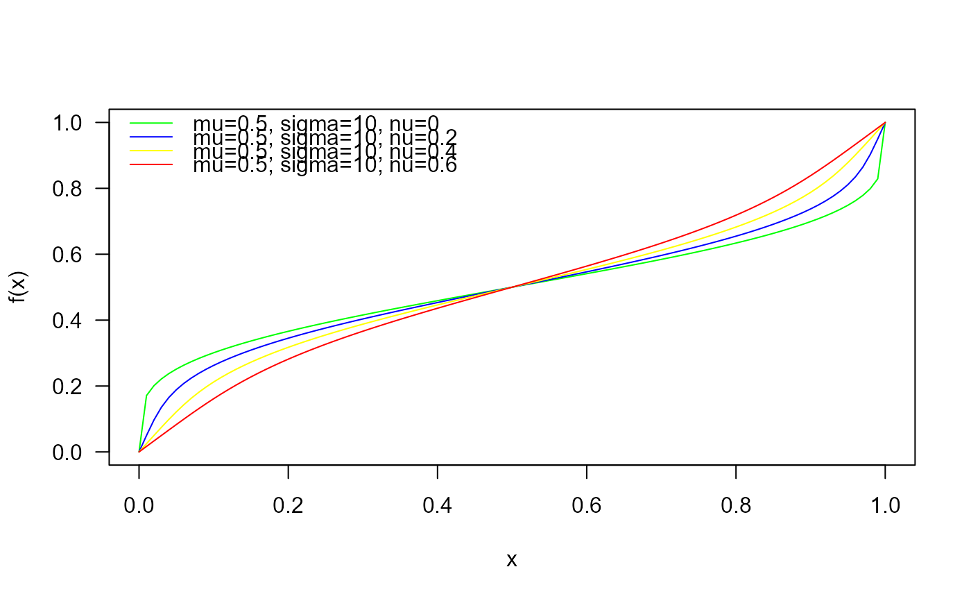
# Example 1
# Plotting the density function for different parameter values
curve(dBER(x, mu=0.5, sigma=10, nu=0),
from=0, to=1, col="green", las=1, ylab="f(x)")
curve(dBER(x, mu=0.5, sigma=10, nu=0.2),
add=TRUE, col= "blue1")
curve(dBER(x, mu=0.5, sigma=10, nu=0.4),
add=TRUE, col="yellow")
curve(dBER(x, mu=0.5, sigma=10, nu=0.6),
add=TRUE, col="red")
legend("topleft", col=c("green", "blue1", "yellow", "red"),
lty=1, bty="n",
legend=c("mu=0.5, sigma=10, nu=0",
"mu=0.5, sigma=10, nu=0.2",
"mu=0.5, sigma=10, nu=0.4",
"mu=0.5, sigma=10, nu=0.6"))
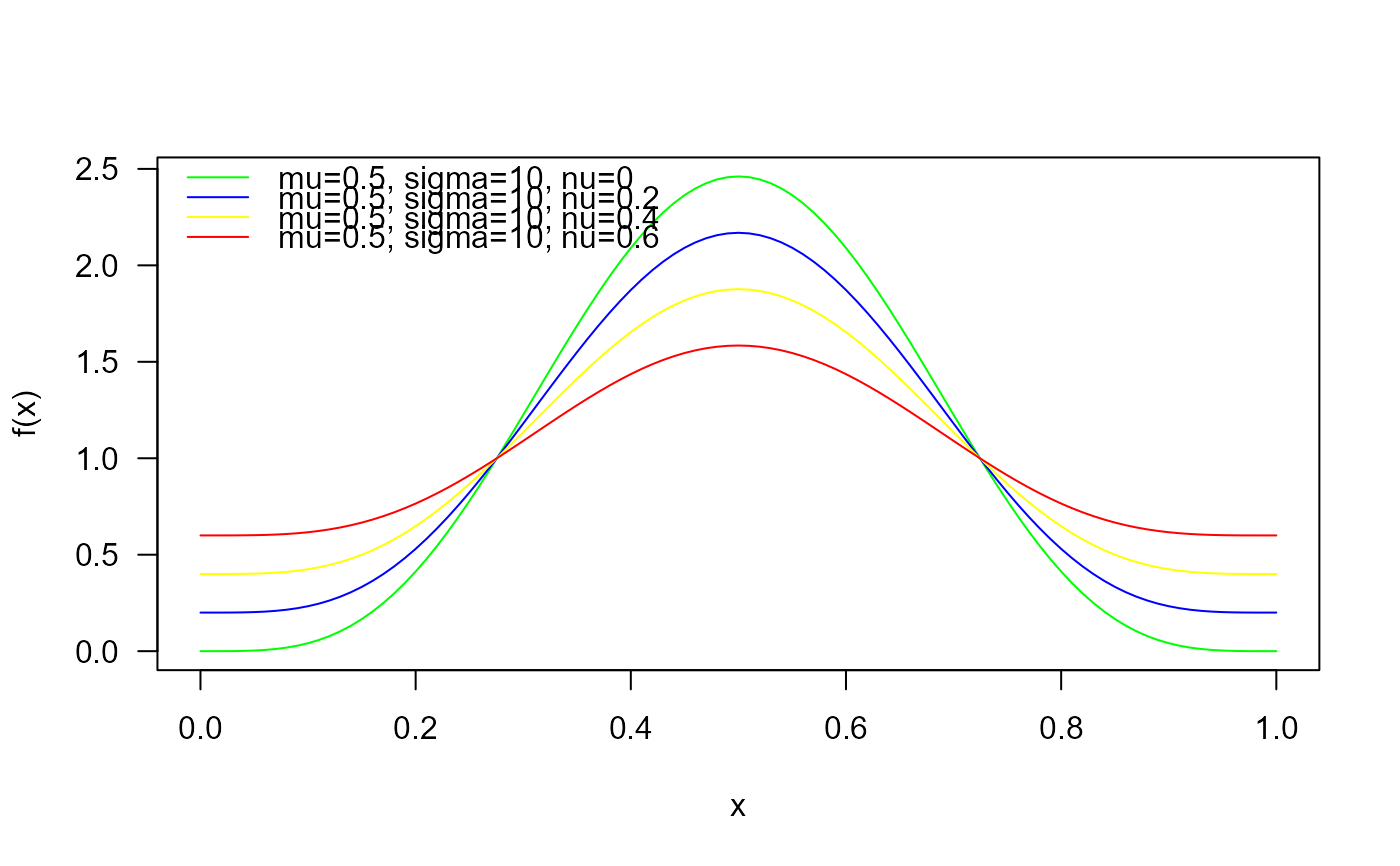 curve(dBER(x, mu=0.3, sigma=10, nu=0),
from=0, to=1, col="green", las=1, ylab="f(x)")
curve(dBER(x, mu=0.3, sigma=10, nu=0.2),
add=TRUE, col= "blue1")
curve(dBER(x, mu=0.3, sigma=10, nu=0.4),
add=TRUE, col="yellow")
curve(dBER(x, mu=0.3, sigma=10, nu=0.6),
add=TRUE, col="red")
legend("topright", col=c("green", "blue1", "yellow", "red"),
lty=1, bty="n",
legend=c("mu=0.5, sigma=10, nu=0",
"mu=0.5, sigma=10, nu=0.2",
"mu=0.5, sigma=10, nu=0.4",
"mu=0.5, sigma=10, nu=0.6"))
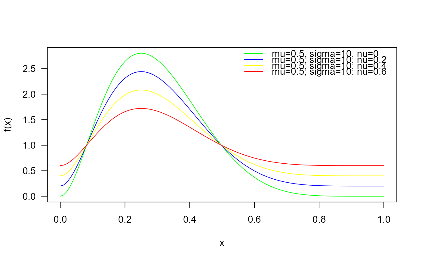
curve(dBER(x, mu=0.3, sigma=10, nu=0),
from=0, to=1, col="green", las=1, ylab="f(x)")
curve(dBER(x, mu=0.3, sigma=10, nu=0.2),
add=TRUE, col= "blue1")
curve(dBER(x, mu=0.3, sigma=10, nu=0.4),
add=TRUE, col="yellow")
curve(dBER(x, mu=0.3, sigma=10, nu=0.6),
add=TRUE, col="red")
legend("topright", col=c("green", "blue1", "yellow", "red"),
lty=1, bty="n",
legend=c("mu=0.5, sigma=10, nu=0",
"mu=0.5, sigma=10, nu=0.2",
"mu=0.5, sigma=10, nu=0.4",
"mu=0.5, sigma=10, nu=0.6"))
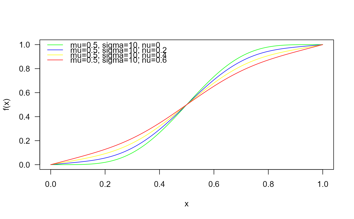
 # Example 2
# Checking if the cumulative curves converge to 1
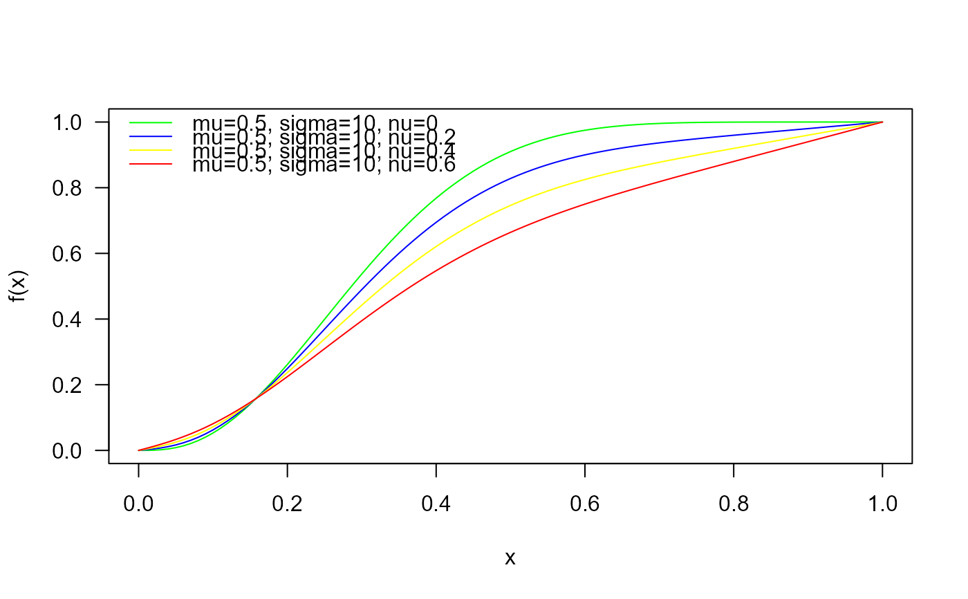
curve(pBER(x, mu=0.5, sigma=10, nu=0),
from=0, to=1, col="green", las=1, ylab="f(x)")
curve(pBER(x, mu=0.5, sigma=10, nu=0.2),
add=TRUE, col= "blue1")
curve(pBER(x, mu=0.5, sigma=10, nu=0.4),
add=TRUE, col="yellow")
curve(pBER(x, mu=0.5, sigma=10, nu=0.6),
add=TRUE, col="red")
legend("topleft", col=c("green", "blue1", "yellow", "red"),
lty=1, bty="n",
legend=c("mu=0.5, sigma=10, nu=0",
"mu=0.5, sigma=10, nu=0.2",
"mu=0.5, sigma=10, nu=0.4",
"mu=0.5, sigma=10, nu=0.6"))
# Example 2
# Checking if the cumulative curves converge to 1
curve(pBER(x, mu=0.5, sigma=10, nu=0),
from=0, to=1, col="green", las=1, ylab="f(x)")
curve(pBER(x, mu=0.5, sigma=10, nu=0.2),
add=TRUE, col= "blue1")
curve(pBER(x, mu=0.5, sigma=10, nu=0.4),
add=TRUE, col="yellow")
curve(pBER(x, mu=0.5, sigma=10, nu=0.6),
add=TRUE, col="red")
legend("topleft", col=c("green", "blue1", "yellow", "red"),
lty=1, bty="n",
legend=c("mu=0.5, sigma=10, nu=0",
"mu=0.5, sigma=10, nu=0.2",
"mu=0.5, sigma=10, nu=0.4",
"mu=0.5, sigma=10, nu=0.6"))
 # Example 3
# Checking the quantile function
mu <- 0.5
sigma <- 10
nu <- 0.4
p <- seq(from=0.01, to=0.99, length.out=100)
plot(x=qBER(p, mu=mu, sigma=sigma, nu=nu), y=p,
xlab="Quantile", las=1, ylab="Probability")
curve(pBER(x, mu=mu, sigma=sigma, nu=nu), add=TRUE, col="red")
# Example 3
# Checking the quantile function
mu <- 0.5
sigma <- 10
nu <- 0.4
p <- seq(from=0.01, to=0.99, length.out=100)
plot(x=qBER(p, mu=mu, sigma=sigma, nu=nu), y=p,
xlab="Quantile", las=1, ylab="Probability")
curve(pBER(x, mu=mu, sigma=sigma, nu=nu), add=TRUE, col="red")
 # Example 4
# Comparing the random generator output with
# the theoretical density
x <- rBER(n= 10000, mu=0.5, sigma=10, nu=0.1)
hist(x, freq=FALSE)
curve(dBER(x, mu=0.5, sigma=10, nu=0.1),
col="tomato", add=TRUE)
# Example 4
# Comparing the random generator output with
# the theoretical density
x <- rBER(n= 10000, mu=0.5, sigma=10, nu=0.1)
hist(x, freq=FALSE)
curve(dBER(x, mu=0.5, sigma=10, nu=0.1),
col="tomato", add=TRUE)