Initial values and search region for Odd Weibull distribution

This function can be used so as to get suggestions about initial values and the search region for parameter estimation in OW distribution.

Usage

initValuesOW(
  formula,
  data = NULL,
  local_reg = loess.options(),
  interpolation = interp.options(),
  ...
)

Arguments

formula: an object of class formula with the response on the left of an operator ~. The right side must be 1.
data: an optional data frame containing the response variables. If data is not specified, the variables are taken from the environment from which initValuesOW is called.
local_reg: a list of control parameters for LOESS. See loess.options.
interpolation: a list of control parameters for interpolation function. See interp.options.
...: further arguments passed to TTTE_Analytical.

Value

Returns an object of class c("initValOW", "HazardShape") containing:

sigma.start value for \(sigma\) parameter of OW distribution.
nu.start value for \(nu\) parameter of OW distribution.
sigma.valid search region for \(sigma\) parameter of OW distribution.
nu.valid search region for \(nu\) parameter of OW distribution.
TTTplot Total Time on Test transform computed from the data.
hazard_type shape of the hazard function determined from the TTT plot.

Details

This function performs a non-parametric estimation of the empirical total time on test (TTT) plot. Then, this estimated curve can be used so as to get suggestions about initial values and the search region for parameters based on hazard shape associated to the shape of empirical TTT plot.

Author

Jaime Mosquera Gutiérrez jmosquerag@unal.edu.co

Examples

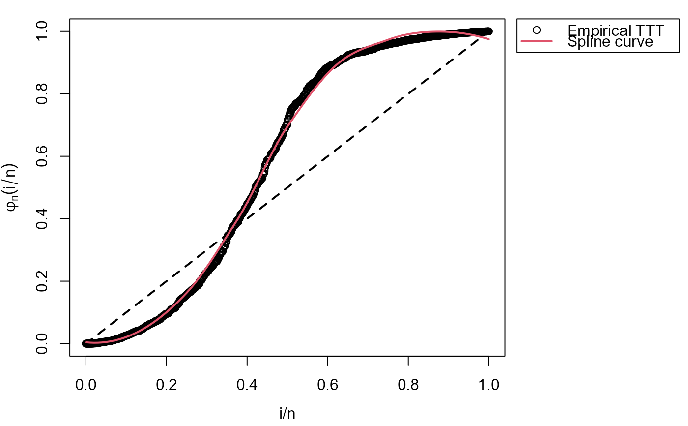
# Example 1
# Bathtuh hazard and its corresponding TTT plot
y1 <- rOW(n = 1000, mu = 0.1, sigma = 7, nu = 0.08)
my_initial_guess1 <- initValuesOW(formula=y1~1)
summary(my_initial_guess1)
#> --------------------------------------------------------------------
#> Initial Values
#> sigma = 5
#> nu = 0.1
#> --------------------------------------------------------------------
#> Search Regions
#> For sigma: all(sigma > 1)
#> For nu: all(nu < 1/sigma)
#> --------------------------------------------------------------------
#> Hazard shape: Bathtub
plot(my_initial_guess1, par_plot=list(mar=c(3.7,3.7,1,2.5),
                                     mgp=c(2.5,1,0)))
#> Warning: The `par_plot` argument of `plot.HazardShape()` is deprecated as of
#> EstimationTools 4.0.0.
#> ℹ Please use `plot.HazardShape()` instead.


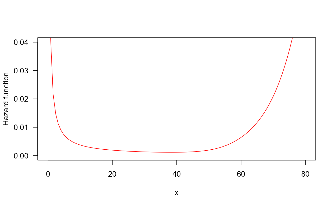
curve(hOW(x, mu = 0.022, sigma = 8, nu = 0.01), from = 0, 
      to = 80, ylim = c(0, 0.04), col = "red", 
      ylab = "Hazard function", las = 1)


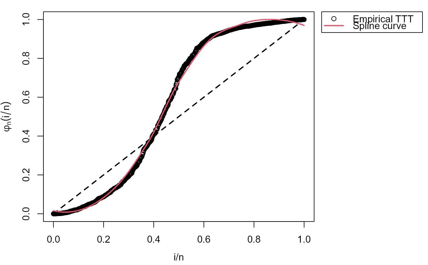
# Example 2
# Bathtuh hazard and its corresponding TTT plot with right censored data
# \donttest{
y2 <- rOW(n = 1000, mu = 0.1, sigma = 7, nu = 0.08)
status <- c(rep(1, 980), rep(0, 20))
my_initial_guess2 <- initValuesOW(formula=Surv(y2, status)~1)
summary(my_initial_guess2)
#> --------------------------------------------------------------------
#> Initial Values
#> sigma = 5
#> nu = 0.1
#> --------------------------------------------------------------------
#> Search Regions
#> For sigma: all(sigma > 1)
#> For nu: all(nu < 1/sigma)
#> --------------------------------------------------------------------
#> Hazard shape: Bathtub
plot(my_initial_guess2, par_plot=list(mar=c(3.7,3.7,1,2.5),
                                     mgp=c(2.5,1,0)))


curve(hOW(x, mu = 0.022, sigma = 8, nu = 0.01), from = 0, 
      to = 80, ylim = c(0, 0.04), col = "red", 
      ylab = "Hazard function", las = 1)

# }