These functions define the density, distribution function, quantile function and random generation for the Wald distribution with parameter \(\mu\) and \(\sigma\).
Usage
dWALD(x, mu, sigma, log = FALSE)

pWALD(q, mu, sigma, lower.tail = TRUE, log.p = FALSE)

qWALD(p, mu, sigma, lower.tail = TRUE, log.p = FALSE)

rWALD(n, mu, sigma)
Arguments
- x, q
vector of (non-negative integer) quantiles.
- mu
vector of the mu parameter.
- sigma
vector of the sigma parameter.
- log, log.p
logical; if TRUE, probabilities p are given as log(p).
- lower.tail
logical; if TRUE (default), probabilities are P[X <= x], otherwise, P[X > x].
- p
vector of probabilities.
- n
number of random values to return.
Value
dWALD gives the density, pWALD gives the distribution
function, qWALD gives the quantile function, rWALD
generates random deviates.
Details
The Wald distribution with parameters \(\mu\) and \(\sigma\) has density given by
\(f(x |\mu, \sigma)=\frac{\sigma}{\sqrt{2 \pi x^3}} \exp \left[-\frac{(\sigma-\mu x)^2}{2x}\right ],\)
for \(x < 0\).
References
Heathcote, A. (2004). Fitting Wald and ex-Wald distributions to response time data: An example using functions for the S-PLUS package. Behavior Research Methods, Instruments, & Computers, 36, 678-694.
Author
Sofia Cuartas, scuartasg@unal.edu.co
Examples
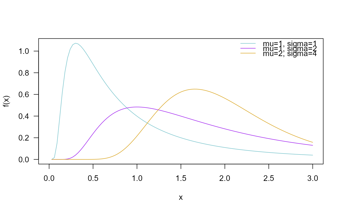
# Example 1
# Plotting the mass function for different parameter values
curve(dWALD(x, mu=1, sigma=1),
from=0, to=3, col="cadetblue3", las=1, ylab="f(x)")
curve(dWALD(x, mu=1, sigma=2),
add=TRUE, col= "purple")
curve(dWALD(x, mu=2, sigma=4),
add=TRUE, col="goldenrod")
legend("topright", col=c("cadetblue3", "purple", "goldenrod"),
lty=1, bty="n",
legend=c("mu=1, sigma=1",
"mu=1, sigma=2",
"mu=2, sigma=4"))
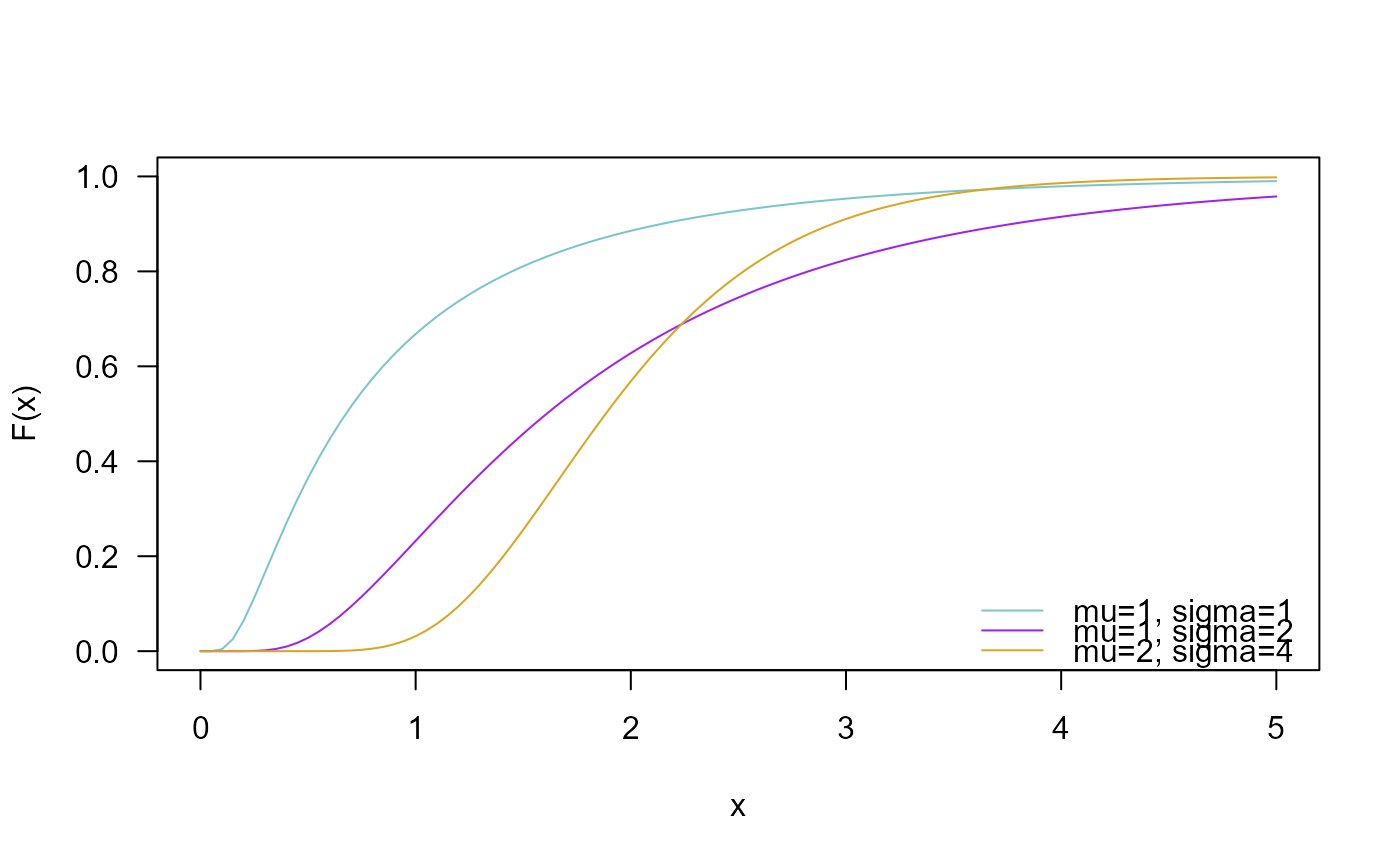
 # Example 2
# Checking if the cumulative curves converge to 1
curve(pWALD(x, mu=1, sigma=1), ylim=c(0, 1),
from=0, to=5, col="cadetblue3", las=1, ylab="F(x)")
curve(pWALD(x, mu=1, sigma=2),
add=TRUE, col= "purple")
curve(pWALD(x, mu=2, sigma=4),
add=TRUE, col="goldenrod")
legend("bottomright", col=c("cadetblue3", "purple", "goldenrod"),
lty=1, bty="n",
legend=c("mu=1, sigma=1",
"mu=1, sigma=2",
"mu=2, sigma=4"))
# Example 2
# Checking if the cumulative curves converge to 1
curve(pWALD(x, mu=1, sigma=1), ylim=c(0, 1),
from=0, to=5, col="cadetblue3", las=1, ylab="F(x)")
curve(pWALD(x, mu=1, sigma=2),
add=TRUE, col= "purple")
curve(pWALD(x, mu=2, sigma=4),
add=TRUE, col="goldenrod")
legend("bottomright", col=c("cadetblue3", "purple", "goldenrod"),
lty=1, bty="n",
legend=c("mu=1, sigma=1",
"mu=1, sigma=2",
"mu=2, sigma=4"))
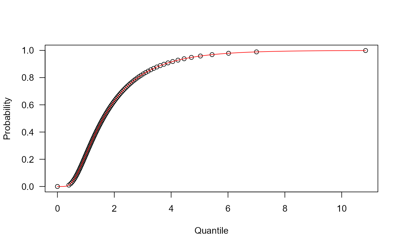
 # Example 3
# Checking the quantile function
mu <- 1
sigma <- 2
p <- seq(from=0, to=0.999, length.out=100)
plot(x=qWALD(p, mu=mu, sigma=sigma), y=p, xlab="Quantile",
las=1, ylab="Probability")
curve(pWALD(x, mu=mu, sigma=sigma), from=0, add=TRUE, col="red")
# Example 3
# Checking the quantile function
mu <- 1
sigma <- 2
p <- seq(from=0, to=0.999, length.out=100)
plot(x=qWALD(p, mu=mu, sigma=sigma), y=p, xlab="Quantile",
las=1, ylab="Probability")
curve(pWALD(x, mu=mu, sigma=sigma), from=0, add=TRUE, col="red")
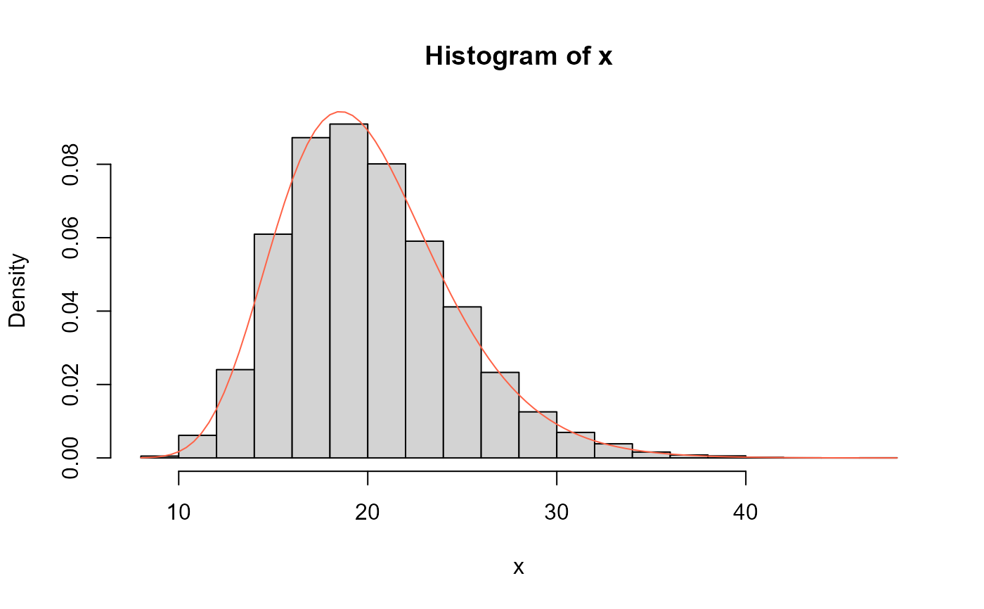
 # Example 4
# Comparing the random generator output with
# the theoretical probabilities
mu <- 1
sigma <- 20
x <- rWALD(n=10000, mu=mu, sigma=sigma)
hist(x, freq=FALSE)
curve(dWALD(x, mu=mu, sigma=sigma), col="tomato", add=TRUE)
# Example 4
# Comparing the random generator output with
# the theoretical probabilities
mu <- 1
sigma <- 20
x <- rWALD(n=10000, mu=mu, sigma=sigma)
hist(x, freq=FALSE)
curve(dWALD(x, mu=mu, sigma=sigma), col="tomato", add=TRUE)