Density, distribution function, quantile function,
random generation and hazard function for the two-parameter
New Exponentiated Exponential with
parameters mu and sigma.
Usage
dNEE(x, mu = 1, sigma = 1, log = FALSE)

pNEE(q, mu = 1, sigma = 1, lower.tail = TRUE, log.p = FALSE)

qNEE(p, mu = 1, sigma = 1, lower.tail = TRUE, log.p = FALSE)

rNEE(n = 1, mu = 1, sigma = 1)

hNEE(x, mu, sigma, log = FALSE)Value
dNEE gives the density, pNEE gives the distribution
function, qNEE gives the quantile function, rNEE
generates random deviates and hNEE gives the hazard function.
Details
The New Exponentiated Exponential distribution with parameters mu
and sigma has density given by
\(f(x | \mu, \sigma) = \log(2^\sigma) \mu \exp(-\mu x) (1-\exp(-\mu x))^{\sigma-1} 2^{(1-\exp(-\mu x))^\sigma}, \)
for \(x>0\), \(\mu>0\) and \(\sigma>0\).
Note: In this implementation we changed the original parameters \(\theta\) for \(\mu\) and \(\alpha\) for \(\sigma\), we did it to implement this distribution within gamlss framework.
References
Hassan, Anwar, I. H. Dar, and M. A. Lone. "A New Class of Probability Distributions With An Application to Engineering Data." Pakistan Journal of Statistics and Operation Research 20.2 (2024): 217-231.
Author
Juliana Garcia, juliana.garciav@udea.edu.co
Examples
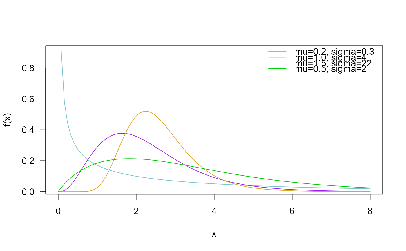
# Example 1
# Plotting the mass function for different parameter values
curve(dNEE(x, mu=0.2, sigma=0.3),
from=0, to=8, col="cadetblue3", las=1, ylab="f(x)")
curve(dNEE(x, mu=1, sigma=4),
add=TRUE, col= "purple")
curve(dNEE(x, mu=1.5, sigma=22),
add=TRUE, col="goldenrod")
curve(dNEE(x, mu=0.5, sigma=2),
add=TRUE, col="green3")
legend("topright", col=c("cadetblue3", "purple", "goldenrod", "green3"), lty=1, bty="n",
legend=c("mu=0.2, sigma=0.3",
"mu=1.0, sigma=4",
"mu=1.5, sigma=22",
"mu=0.5, sigma=2"))
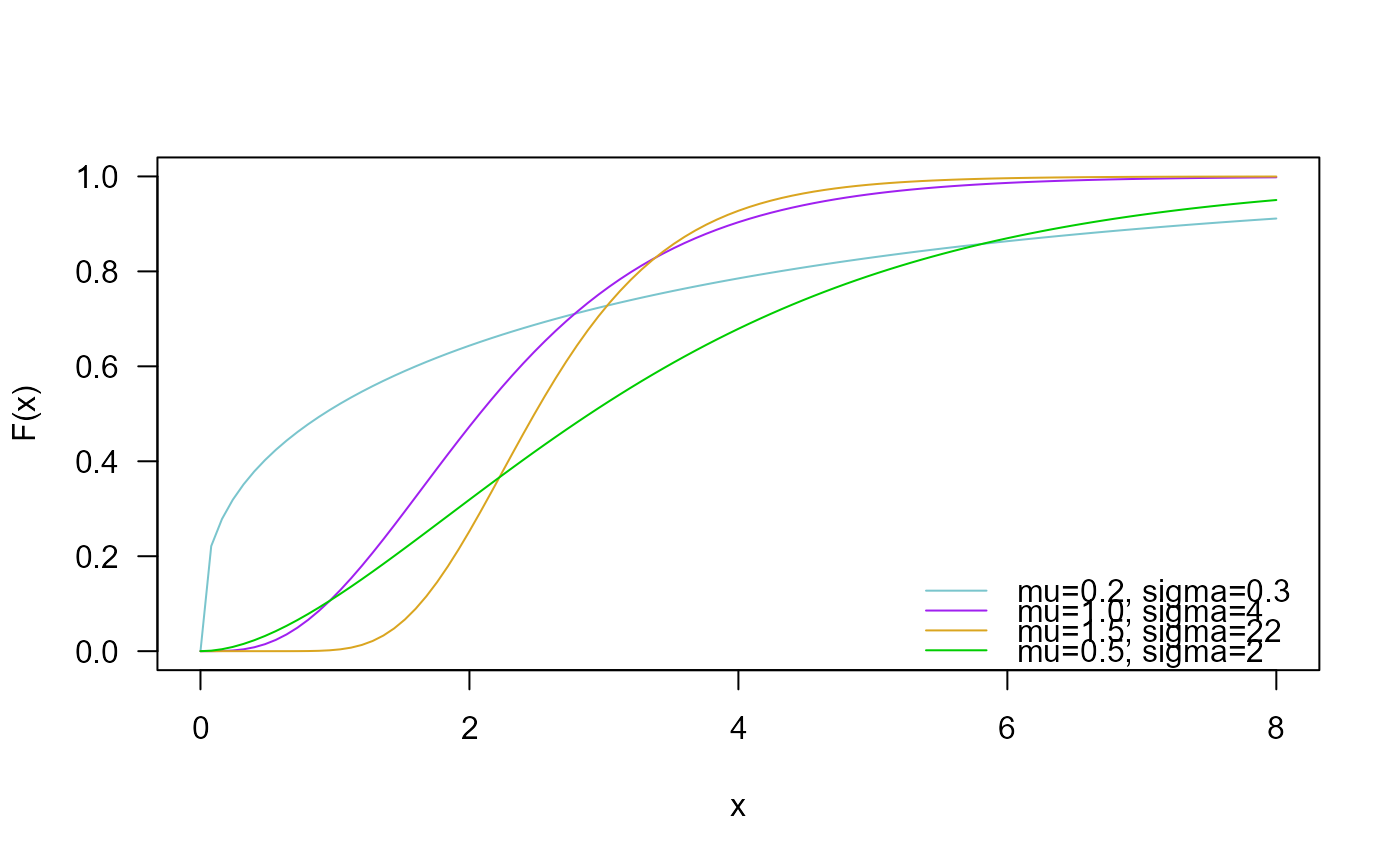
 # Example 2
# Checking if the cumulative curves converge to 1
curve(pNEE(x, mu=0.2, sigma=0.3), ylim=c(0, 1),
from=0, to=8, col="cadetblue3", las=1, ylab="F(x)")
curve(pNEE(x, mu=1, sigma=4),
add=TRUE, col= "purple")
curve(pNEE(x, mu=1.5, sigma=22),
add=TRUE, col="goldenrod")
curve(pNEE(x, mu=0.5, sigma=2),
add=TRUE, col="green3")
legend("bottomright", col=c("cadetblue3", "purple", "goldenrod", "green3"), lty=1, bty="n",
legend=c("mu=0.2, sigma=0.3",
"mu=1.0, sigma=4",
"mu=1.5, sigma=22",
"mu=0.5, sigma=2"))
# Example 2
# Checking if the cumulative curves converge to 1
curve(pNEE(x, mu=0.2, sigma=0.3), ylim=c(0, 1),
from=0, to=8, col="cadetblue3", las=1, ylab="F(x)")
curve(pNEE(x, mu=1, sigma=4),
add=TRUE, col= "purple")
curve(pNEE(x, mu=1.5, sigma=22),
add=TRUE, col="goldenrod")
curve(pNEE(x, mu=0.5, sigma=2),
add=TRUE, col="green3")
legend("bottomright", col=c("cadetblue3", "purple", "goldenrod", "green3"), lty=1, bty="n",
legend=c("mu=0.2, sigma=0.3",
"mu=1.0, sigma=4",
"mu=1.5, sigma=22",
"mu=0.5, sigma=2"))
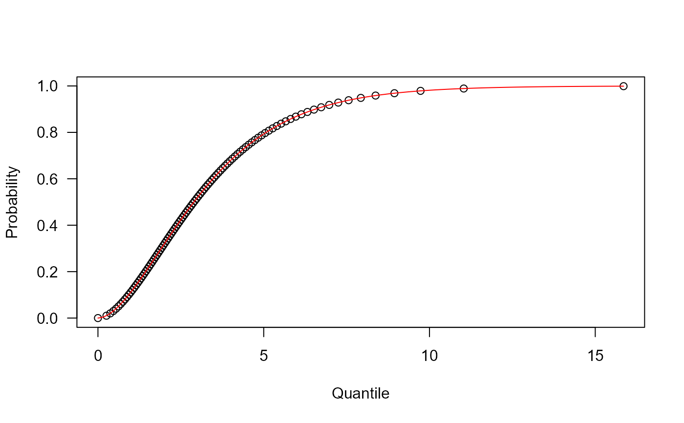
 # Example 3
# Checking the quantile function
mu <- 0.5
sigma <- 2
p <- seq(from=0, to=0.999, length.out=100)
plot(x=qNEE(p, mu=mu, sigma=sigma), y=p, xlab="Quantile",
las=1, ylab="Probability")
curve(pNEE(x, mu=mu, sigma=sigma), from=0, add=TRUE, col="red")
# Example 3
# Checking the quantile function
mu <- 0.5
sigma <- 2
p <- seq(from=0, to=0.999, length.out=100)
plot(x=qNEE(p, mu=mu, sigma=sigma), y=p, xlab="Quantile",
las=1, ylab="Probability")
curve(pNEE(x, mu=mu, sigma=sigma), from=0, add=TRUE, col="red")
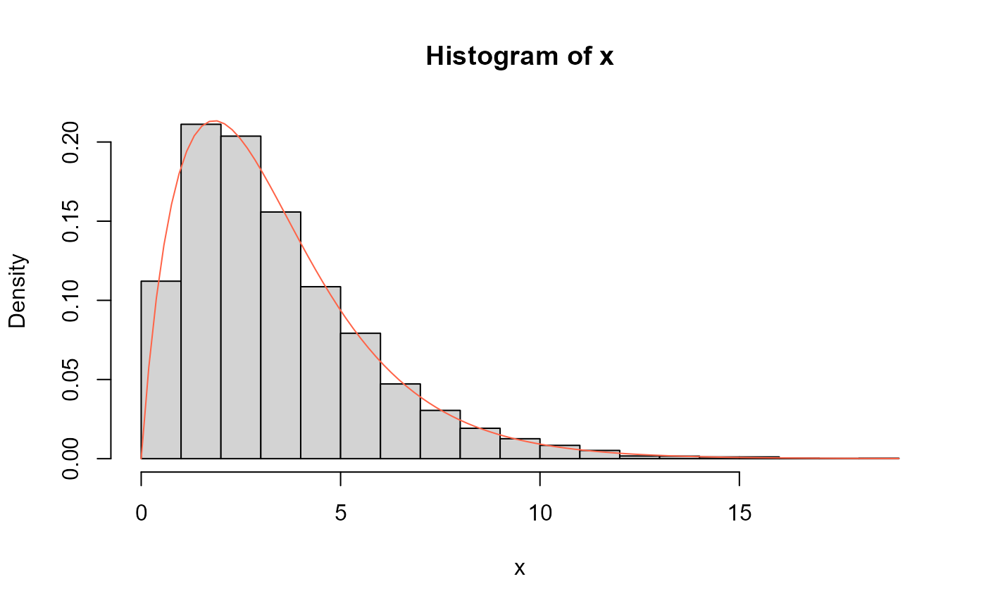
 # Example 4
# Comparing the random generator output with
# the theoretical probabilities
mu <- 0.5
sigma <- 2
x <- rNEE(n=10000, mu=mu, sigma=sigma)
hist(x, freq=FALSE)
curve(dNEE(x, mu=mu, sigma=sigma), col="tomato", add=TRUE)
# Example 4
# Comparing the random generator output with
# the theoretical probabilities
mu <- 0.5
sigma <- 2
x <- rNEE(n=10000, mu=mu, sigma=sigma)
hist(x, freq=FALSE)
curve(dNEE(x, mu=mu, sigma=sigma), col="tomato", add=TRUE)