Density, distribution function, quantile function,
random generation and hazard function for the Gamma Weibull distribution
with parameters mu, sigma, nu and tau.
Usage
dGammaW(x, mu, sigma, nu, log = FALSE)

pGammaW(q, mu, sigma, nu, lower.tail = TRUE, log.p = FALSE)

qGammaW(p, mu, sigma, nu, lower.tail = TRUE, log.p = FALSE)

rGammaW(n, mu, sigma, nu)

hGammaW(x, mu, sigma, nu)Value
dGammaW gives the density, pGammaW gives the distribution
function, qGammaW gives the quantile function, rGammaW
generates random deviates and hGammaW gives the hazard function.
Details
The Gamma Weibull Distribution with parameters mu,
sigma and nu has density given by
\(f(x)= \frac{\sigma \mu^{\nu}}{\Gamma(\nu)} x^{\nu \sigma - 1} \exp(-\mu x^\sigma),\)
for \(x > 0\), \(\mu > 0\), \(\sigma > 0\) and \(\nu > 0\).
References
Almalki, S. J., & Nadarajah, S. (2014). Modifications of the Weibull distribution: A review. Reliability Engineering & System Safety, 124, 32-55.
Stacy, E. W. (1962). A generalization of the gamma distribution. The Annals of mathematical statistics, 1187-1192.
Author
Johan David Marin Benjumea, johand.marin@udea.edu.co
Examples
# Example 1
# Plotting the mass function for different parameter values
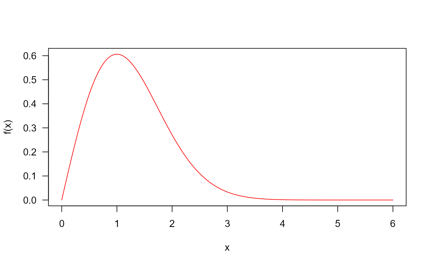
## The probability density function
curve(dGammaW(x, mu=2, sigma=1.5, nu=0.5),
from=0, to=2,
col="red", lwd=2,
main="Density function",
xlab="x", ylab="f(x)")
curve(dGammaW(x, mu=2.4, sigma=1.5, nu=1.3),
col="blue",
lwd=2,
add=TRUE)
legend("topright", legend=c("mu=2.0, sigma=1.5, nu=0.5",
"mu=2.4, sigma=1.5, nu=1.3"),
col=c("red", "blue"), lwd=2, cex=0.6)
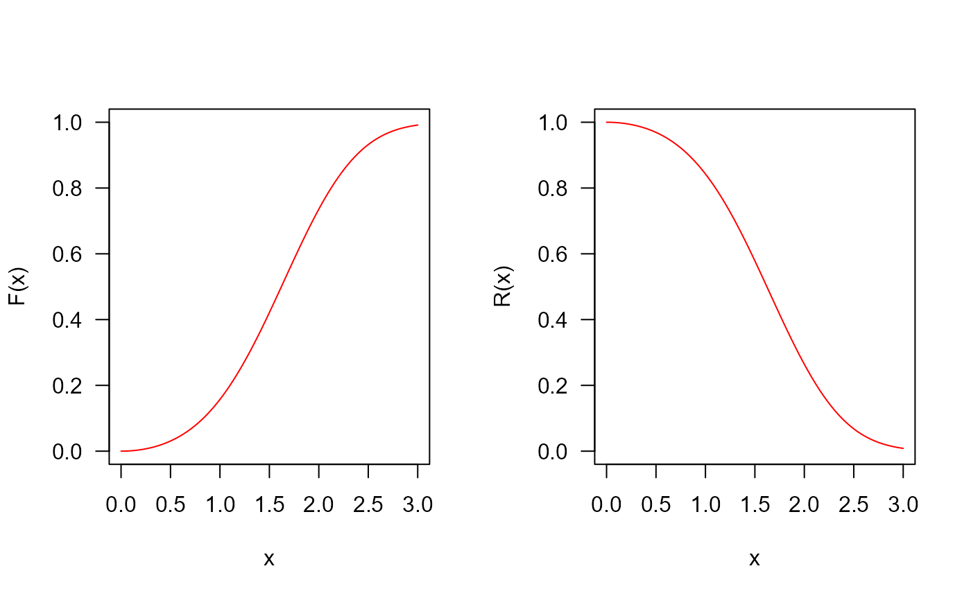
 # Example 2
# Checking if the cumulative curves converge to 1
curve(pGammaW(x, mu=0.5, sigma=2, nu=1),
from=0, to=3,
col="red", lwd=2, ylab="F(x)")
curve(pGammaW(x, mu=2.4, sigma=1.5, nu=1.3),
col="blue",
lwd=2,
add=TRUE)
legend("bottomright", legend=c("mu=2.0, sigma=1.5, nu=0.5",
"mu=2.4, sigma=1.5, nu=1.3"),
col=c("red", "blue"), lwd=2, cex=0.6)
# Example 2
# Checking if the cumulative curves converge to 1
curve(pGammaW(x, mu=0.5, sigma=2, nu=1),
from=0, to=3,
col="red", lwd=2, ylab="F(x)")
curve(pGammaW(x, mu=2.4, sigma=1.5, nu=1.3),
col="blue",
lwd=2,
add=TRUE)
legend("bottomright", legend=c("mu=2.0, sigma=1.5, nu=0.5",
"mu=2.4, sigma=1.5, nu=1.3"),
col=c("red", "blue"), lwd=2, cex=0.6)
 # Example 3
# The quantile function
p <- seq(from=0, to=0.999, length.out=100)
plot(x=qGammaW(p, mu=2.3, sigma=1.7, nu=1.2), y=p, xlab="Quantile",
las=1, ylab="Probability", main="Quantile function ")
curve(pGammaW(x, mu=2.3, sigma=1.7, nu=1.2),
from=0, add=TRUE, col="tomato", lwd=2.5)
# Example 3
# The quantile function
p <- seq(from=0, to=0.999, length.out=100)
plot(x=qGammaW(p, mu=2.3, sigma=1.7, nu=1.2), y=p, xlab="Quantile",
las=1, ylab="Probability", main="Quantile function ")
curve(pGammaW(x, mu=2.3, sigma=1.7, nu=1.2),
from=0, add=TRUE, col="tomato", lwd=2.5)
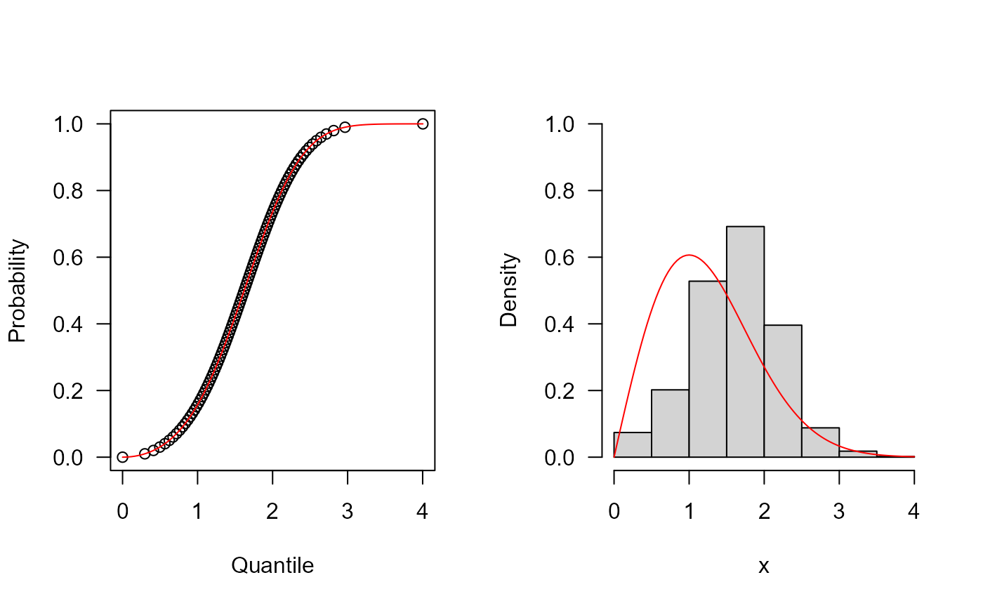 # Example 4
# The random function
x <- rGammaW(n=10000, mu=2.4, sigma=1.5, nu=1.3)
hist(x, freq=FALSE)
curve(dGammaW(x, mu=2.4, sigma=1.5, nu=1.3),
add=TRUE, col="tomato", lwd=2)
# Example 4
# The random function
x <- rGammaW(n=10000, mu=2.4, sigma=1.5, nu=1.3)
hist(x, freq=FALSE)
curve(dGammaW(x, mu=2.4, sigma=1.5, nu=1.3),
add=TRUE, col="tomato", lwd=2)
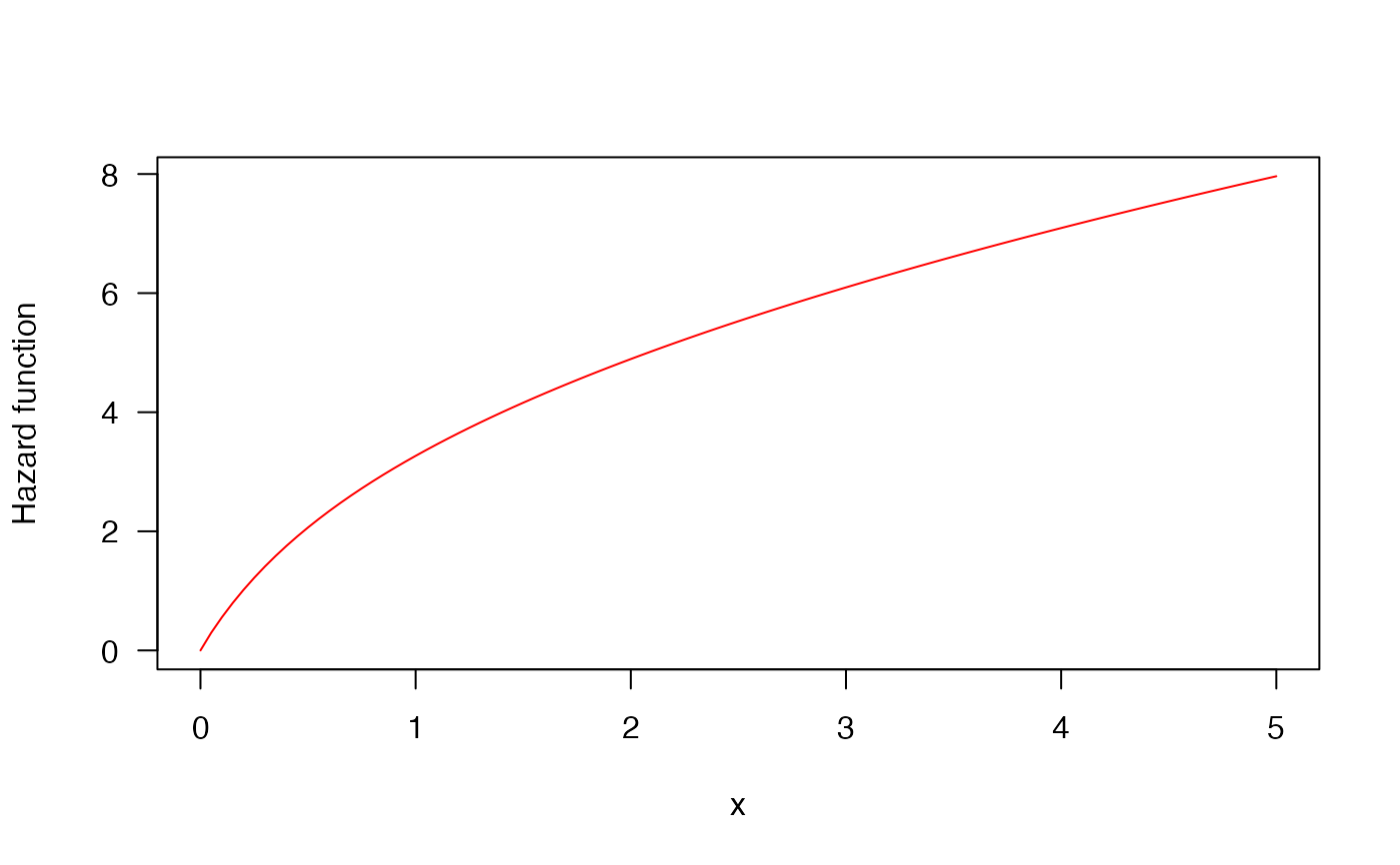
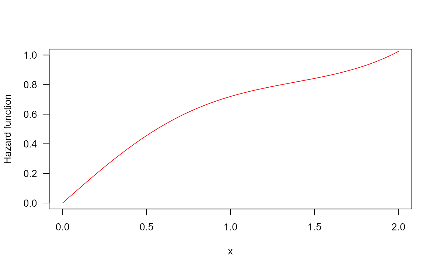 # The Hazard function
curve(hGammaW(x, mu=2.4, sigma=1.5, nu=1.3), from=0, to=5,
col="red", ylab="Hazard function", las=1)
# The Hazard function
curve(hGammaW(x, mu=2.4, sigma=1.5, nu=1.3), from=0, to=5,
col="red", ylab="Hazard function", las=1)