These functions define the density, distribution function, quantile function and random generation for the Generalized Lindley Type II, GLIN(), distribution with parameters \(\mu\) and \(\sigma\).
Usage
dGLIN(x, mu, sigma, log = FALSE)

pGLIN(q, mu, sigma, lower.tail = TRUE, log.p = FALSE)

qGLIN(p, mu, sigma, lower.tail = TRUE, log.p = FALSE)

rGLIN(n, mu, sigma)

hGLIN(x, mu = 0.5, sigma = 0.5)
Arguments
- x, q
vector of positive quantiles.
- mu
vector of the mu parameter.
- sigma
vector of the sigma parameter.
- log, log.p
logical; if TRUE, probabilities p are given as log(p).
- lower.tail
logical; if TRUE (default), probabilities are \(P[X \le x]\), otherwise, \(P[X > x]\).
- p
vector of probabilities.
- n
number of random values to return.
Value
dGLIN gives the density, pGLIN gives the distribution
function, qGLIN gives the quantile function, and
rGLIN generates random deviates.
Details
The Generalized Lindley Type II distribution with parameters
mu and sigma has probability density function
\( f(x|\mu,\sigma)= \frac{\mu^2}{\mu+1} \left( 1+\frac{\mu^{\sigma-2}x^{\sigma-1}} {\Gamma(\sigma)} \right) e^{-\mu x}, \)
for \(x>0\), \(\mu>0\) and \(\sigma>0\).
The distribution is a two-parameter extension of the classical Lindley distribution and belongs to the class of finite mixtures involving exponential and gamma components. It provides additional flexibility for modeling positively skewed lifetime data.
The original parameters of the distribution are denoted by \(\theta\) and \(\alpha\). In the GAMLSS implementation, they are re-parameterized as \(\mu=\theta\) and \(\sigma=\alpha\).
The \(r\)-th raw moment is given by
\( E(X^r)= \frac{1} {\mu^r(\mu+1)} \left[ \mu\Gamma(r+1) + \frac{\Gamma(r+\sigma)} {\Gamma(\sigma)} \right]. \)
In particular, the mean is
\( E(X)= \frac{\mu+\sigma} {\mu(\mu+1)}. \)
and the variance is
\( Var(X)= \frac{\mu^2 + \mu(\sigma^2 - \sigma + 2) + \sigma} {\mu^2(\mu + 1)^2}. \)
The GLIN distribution is a flexible two-parameter extension of the classical Lindley distribution and is suitable for modeling positive lifetime and survival data.
References
Ekhosuehi, N., Opone, F., & Odobaire, F. (2018). A New Generalized Two Parameter Lindley Distribution. Journal of the Nigerian Statistical Association, 30, 547–566.
See also
GLIN.
Author
Sofia Cadavid Rueda, socadavidr@unal.edu.co
Examples
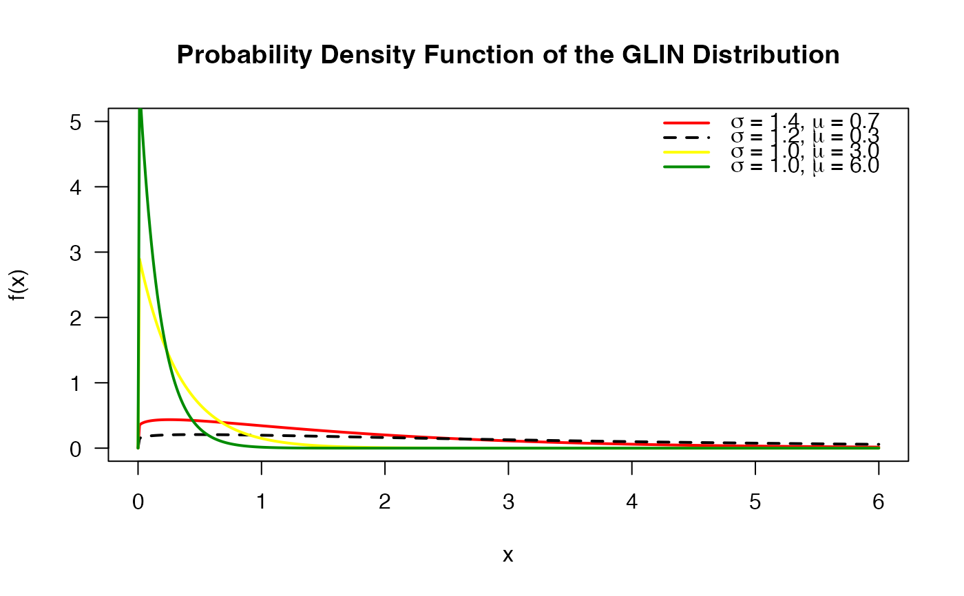
# Example 1
# Plotting the mass function for different parameter values
x_vals <- seq(0, 6, length.out = 500)
# Calculate densities
d1 <- dGLIN(x_vals, mu = 0.7, sigma = 1.4)
d2 <- dGLIN(x_vals, mu = 0.3, sigma = 1.2)
d3 <- dGLIN(x_vals, mu = 3.0, sigma = 1.0)
d4 <- dGLIN(x_vals, mu = 6.0, sigma = 1.0)
# Plot
plot(x_vals, d1, type = "l", col = "red", lwd = 2, lty = 1,
ylim = c(0, 5), xlim = c(0, 6),
xlab = "x", ylab = "f(x)",
main = "Probability Density Function of the GLIN Distribution",
las = 1)
lines(x_vals, d2, col = "black", lwd = 2, lty = 2)
lines(x_vals, d3, col = "yellow", lwd = 2, lty = 1)
lines(x_vals, d4, col = "green4", lwd = 2, lty = 1)
# Legend
legend("topright",
col = c("red", "black", "yellow", "green4"),
lwd = 2,
lty = c(1, 2, 1, 1),
legend = c(expression(paste(sigma, " = 1.4, ", mu, " = 0.7")),
expression(paste(sigma, " = 1.2, ", mu, " = 0.3")),
expression(paste(sigma, " = 1.0, ", mu, " = 3.0")),
expression(paste(sigma, " = 1.0, ", mu, " = 6.0"))),
bty = "n")
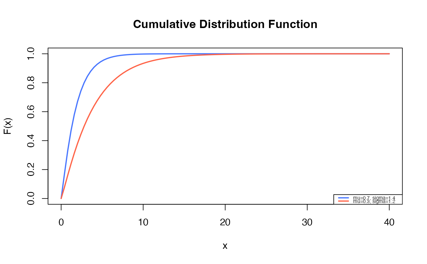
 # Example 2
# Checking if the cumulative curves converge to 1
curve(pGLIN(x, mu=0.7, sigma=1.4),
from=0.00001, to=40,
ylim=c(0, 1),
col="royalblue1", lwd=2,
main="Cumulative Distribution Function",
xlab="x", ylab="F(x)")
curve(pGLIN(x, mu=0.3, sigma=1.2),
col="tomato",
lwd=2,
add=TRUE)
legend("bottomright", legend=c("mu=0.7, sigma=1.4",
"mu=0.3, sigma=1.2"),
col=c("royalblue1", "tomato", "seagreen"), lwd=2, cex=0.5)
# Example 2
# Checking if the cumulative curves converge to 1
curve(pGLIN(x, mu=0.7, sigma=1.4),
from=0.00001, to=40,
ylim=c(0, 1),
col="royalblue1", lwd=2,
main="Cumulative Distribution Function",
xlab="x", ylab="F(x)")
curve(pGLIN(x, mu=0.3, sigma=1.2),
col="tomato",
lwd=2,
add=TRUE)
legend("bottomright", legend=c("mu=0.7, sigma=1.4",
"mu=0.3, sigma=1.2"),
col=c("royalblue1", "tomato", "seagreen"), lwd=2, cex=0.5)
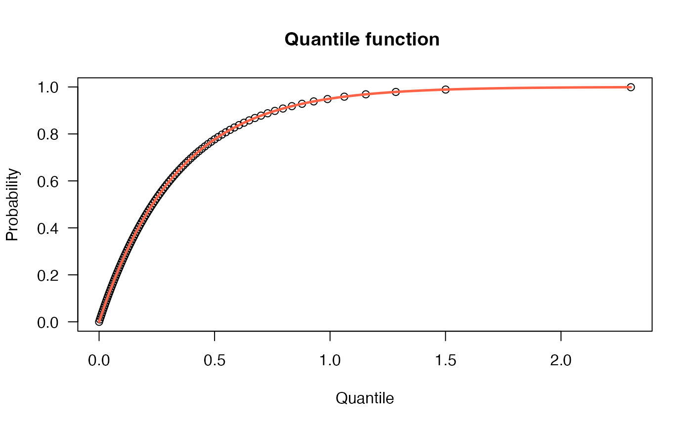
 # Example 3
# The quantile function
p <- seq(from=0, to=0.999, length.out=100)
plot(x=qGLIN(p, mu=3, sigma=1), y=p, xlab="Quantile",
las=1, ylab="Probability", main="Quantile function ")
curve(pGLIN(x, mu=3, sigma=1),
from=0, add=TRUE, col="tomato", lwd=2.5)
# Example 3
# The quantile function
p <- seq(from=0, to=0.999, length.out=100)
plot(x=qGLIN(p, mu=3, sigma=1), y=p, xlab="Quantile",
las=1, ylab="Probability", main="Quantile function ")
curve(pGLIN(x, mu=3, sigma=1),
from=0, add=TRUE, col="tomato", lwd=2.5)
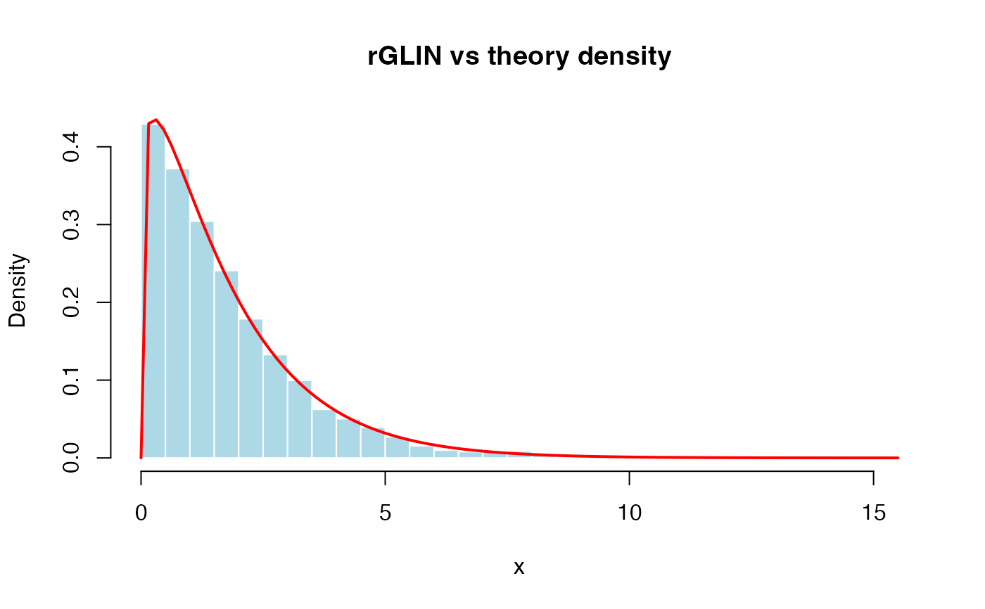
 # Example 4
# The random function
set.seed(123)
x <- rGLIN(5000, mu=0.7, sigma=1.4)
hist(x, breaks=50, freq=FALSE,
main="rGLIN vs theory density",
xlab="x", col="lightblue", border="white")
curve(dGLIN(x, mu=0.7, sigma=1.4),
add=TRUE, col="red", lwd=2)
# Example 4
# The random function
set.seed(123)
x <- rGLIN(5000, mu=0.7, sigma=1.4)
hist(x, breaks=50, freq=FALSE,
main="rGLIN vs theory density",
xlab="x", col="lightblue", border="white")
curve(dGLIN(x, mu=0.7, sigma=1.4),
add=TRUE, col="red", lwd=2)
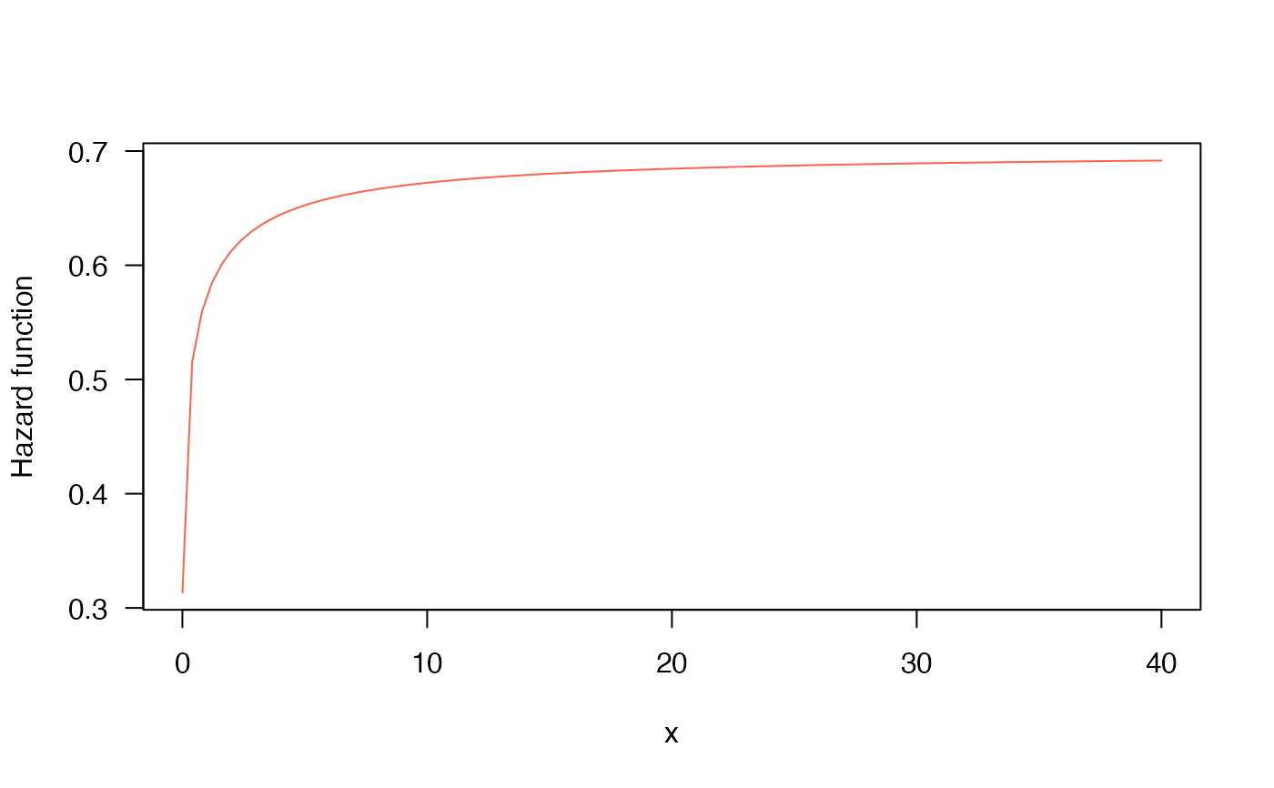
 # Example 5
# The Hazard function
curve(hGLIN(x, mu=0.7, sigma=1.4), from=0.001, to=40,
col="tomato", ylab="Hazard function", las=1)
# Example 5
# The Hazard function
curve(hGLIN(x, mu=0.7, sigma=1.4), from=0.001, to=40,
col="tomato", ylab="Hazard function", las=1)