Density, distribution function, quantile function,
random generation and hazard function for the
gamma original distribution with
parameters mu and sigma.
Usage
dGAo(x, mu = 1, sigma = 1, log = FALSE)

pGAo(q, mu = 1, sigma = 1, lower.tail = TRUE, log.p = FALSE)

qGAo(p, mu = 1, sigma = 1, lower.tail = TRUE, log.p = FALSE)

rGAo(n, mu = 1, sigma = 1)

hGAo(x, mu, sigma)Value
dGAo gives the density, pGAo gives the distribution
function, qGAo gives the quantile function, rGAo
generates random deviates and hGAo gives the hazard function.
Details
The gamma original with parameters mu and sigma
has density given by
\(f(x|\mu,\sigma) = \frac{x^{\mu-1}e^{-x/\sigma}}{\sigma^\mu \Gamma(\mu)}\)
for \(x>0\), \(\mu>0\) and \(\sigma>0\). The parameter \(\mu\) is the shape parameter and \(\sigma\) is the scale parameter. In this parameterization \(\mu\) is the median of \(X\), \(E(X)=\mu \sigma\) and \(Var(X)=\mu \sigma^2\).
References
Abramowitz M, Stegun IA (1972). Handbook of Mathematical Functions with Formulas, Graphs, and Mathematical Tables. Dover Publications, New York. ISBN 0486612724. Chapter 6: Gamma and Related Functions.
See also
GAo.
Examples
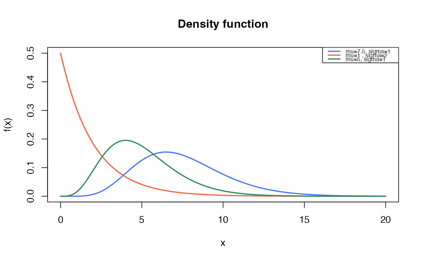
# Example 1
# Plotting the mass function for different parameter values
curve(dGAo(x, mu=7.5, sigma=1),
from=0.001, to=20,
ylim=c(0, 0.5),
col="royalblue1", lwd=2,
main="Density function",
xlab="x", ylab="f(x)")
curve(dGAo(x, mu=1, sigma=2),
col="tomato",
lwd=2,
add=TRUE)
curve(dGAo(x, mu=5, sigma=1),
col="seagreen",
lwd=2,
add=TRUE)
legend("topright", legend=c("mu=7.5, sigma=1",
"mu=1 , sigma=2",
"mu=5, sigma=1"),
col=c("royalblue1", "tomato", "seagreen"), lwd=2, cex=0.6)
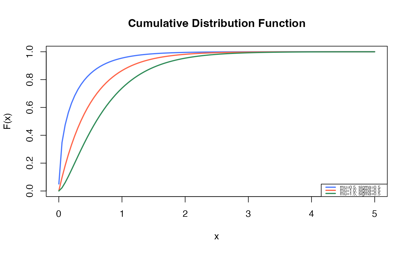
 # Example 2
# Checking if the cumulative curves converge to 1
curve(pGAo(x, mu=0.5, sigma=0.5),
from=0.001, to=5,
ylim=c(0, 1),
col="royalblue1", lwd=2,
main="Cumulative Distribution Function",
xlab="x", ylab="F(x)")
curve(pGAo(x, mu=1, sigma=0.5),
col="tomato",
lwd=2,
add=TRUE)
curve(pGAo(x, mu=1.5, sigma=0.5),
col="seagreen",
lwd=2,
add=TRUE)
legend("bottomright", legend=c("mu=0.5, sigma=0.5",
"mu=1.0, sigma=0.5",
"mu=1.5, sigma=0.5"),
col=c("royalblue1", "tomato", "seagreen"), lwd=2, cex=0.5)
# Example 2
# Checking if the cumulative curves converge to 1
curve(pGAo(x, mu=0.5, sigma=0.5),
from=0.001, to=5,
ylim=c(0, 1),
col="royalblue1", lwd=2,
main="Cumulative Distribution Function",
xlab="x", ylab="F(x)")
curve(pGAo(x, mu=1, sigma=0.5),
col="tomato",
lwd=2,
add=TRUE)
curve(pGAo(x, mu=1.5, sigma=0.5),
col="seagreen",
lwd=2,
add=TRUE)
legend("bottomright", legend=c("mu=0.5, sigma=0.5",
"mu=1.0, sigma=0.5",
"mu=1.5, sigma=0.5"),
col=c("royalblue1", "tomato", "seagreen"), lwd=2, cex=0.5)
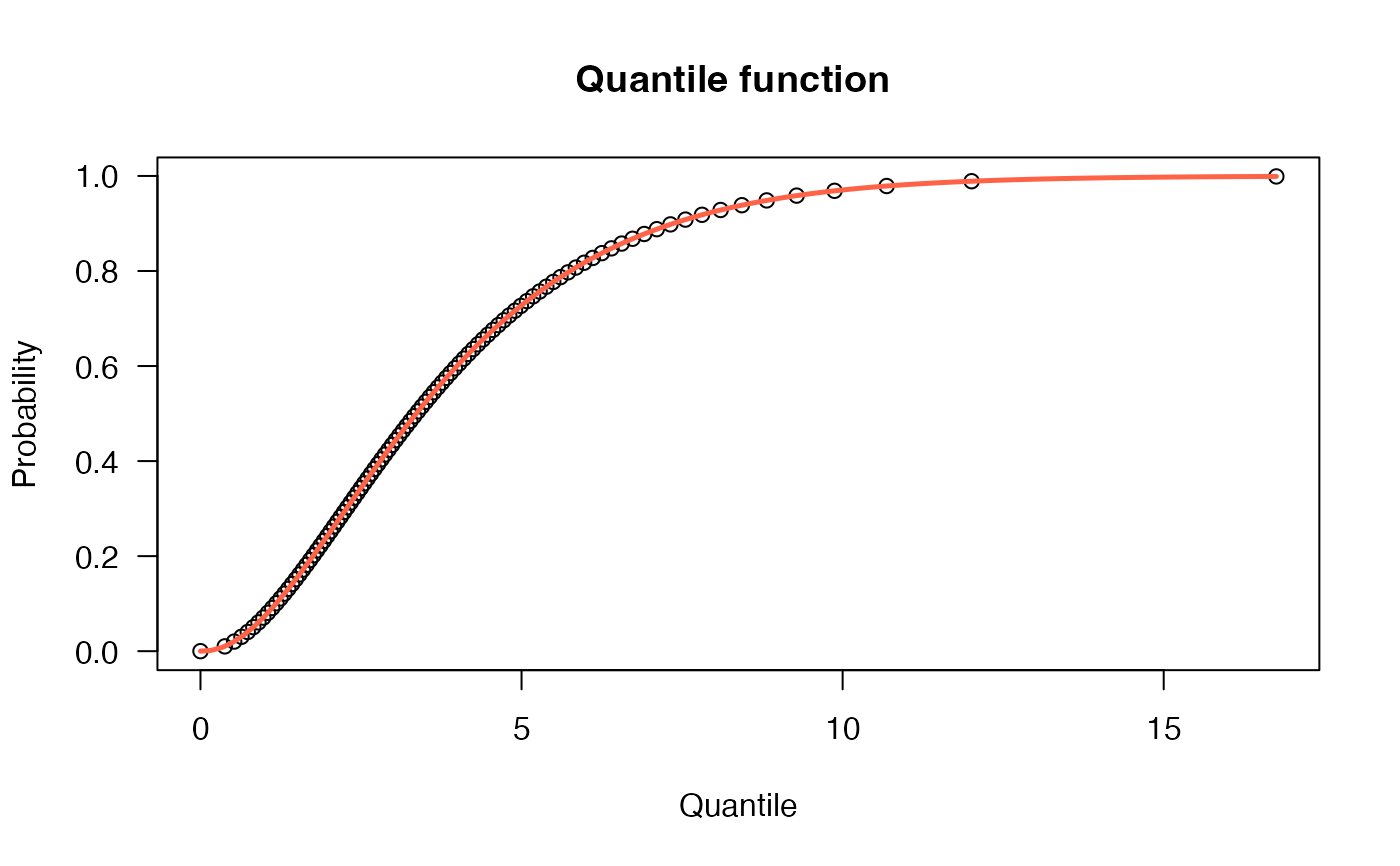
 # Example 3
# The quantile function
p <- seq(from=0, to=0.999, length.out=100)
plot(x=qGAo(p, mu=2.3, sigma=1.7), y=p, xlab="Quantile",
las=1, ylab="Probability", main="Quantile function ")
curve(pGAo(x, mu=2.3, sigma=1.7),
from=0, add=TRUE, col="tomato", lwd=2.5)
# Example 3
# The quantile function
p <- seq(from=0, to=0.999, length.out=100)
plot(x=qGAo(p, mu=2.3, sigma=1.7), y=p, xlab="Quantile",
las=1, ylab="Probability", main="Quantile function ")
curve(pGAo(x, mu=2.3, sigma=1.7),
from=0, add=TRUE, col="tomato", lwd=2.5)
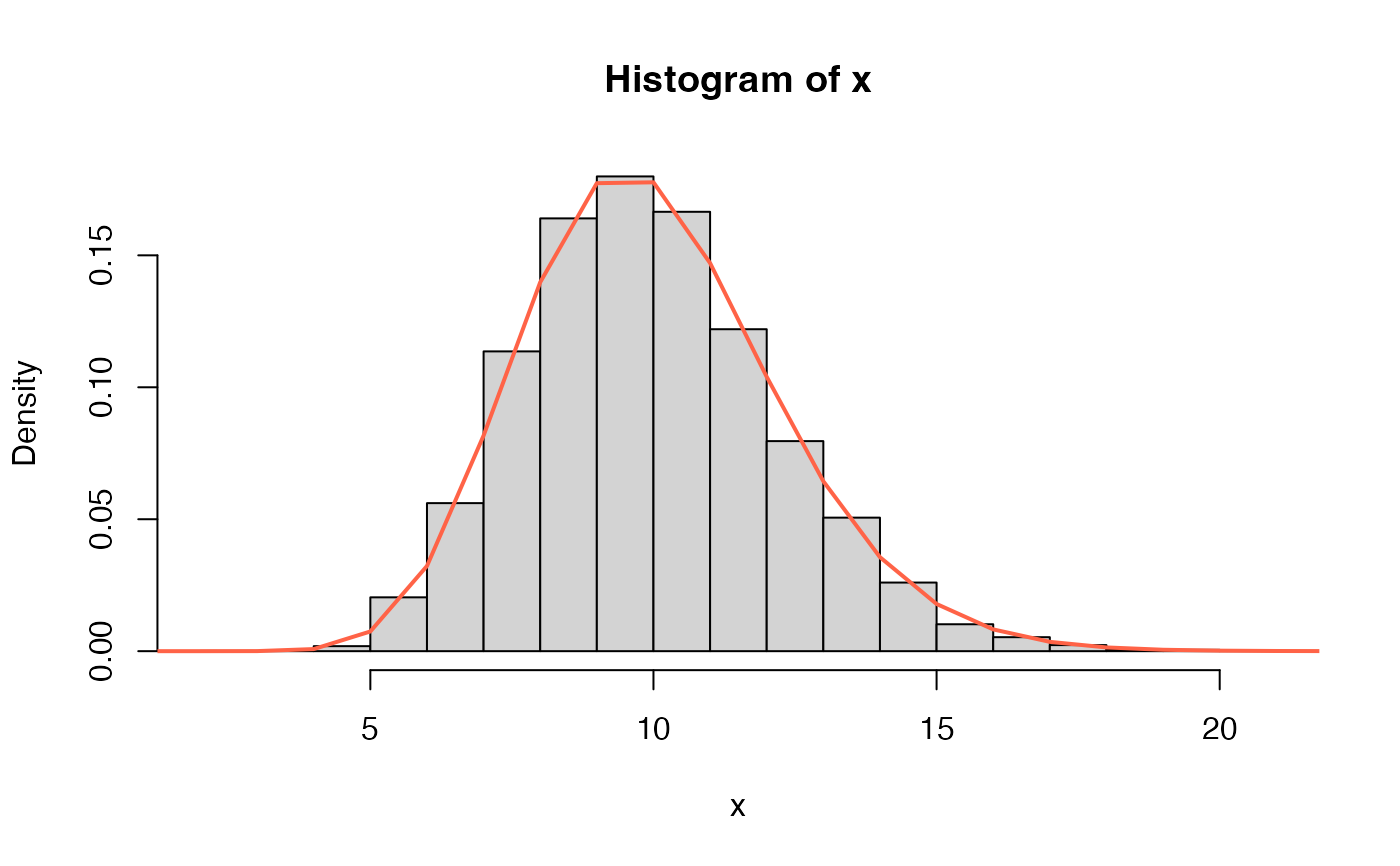
 # Example 4
# The random function
x <- rGAo(n=10000, mu=20, sigma=0.5)
hist(x, freq=FALSE)
curve(dGAo(x, mu=20, sigma=0.5), from=0, to=100,
add=TRUE, col="tomato", lwd=2)
# Example 4
# The random function
x <- rGAo(n=10000, mu=20, sigma=0.5)
hist(x, freq=FALSE)
curve(dGAo(x, mu=20, sigma=0.5), from=0, to=100,
add=TRUE, col="tomato", lwd=2)
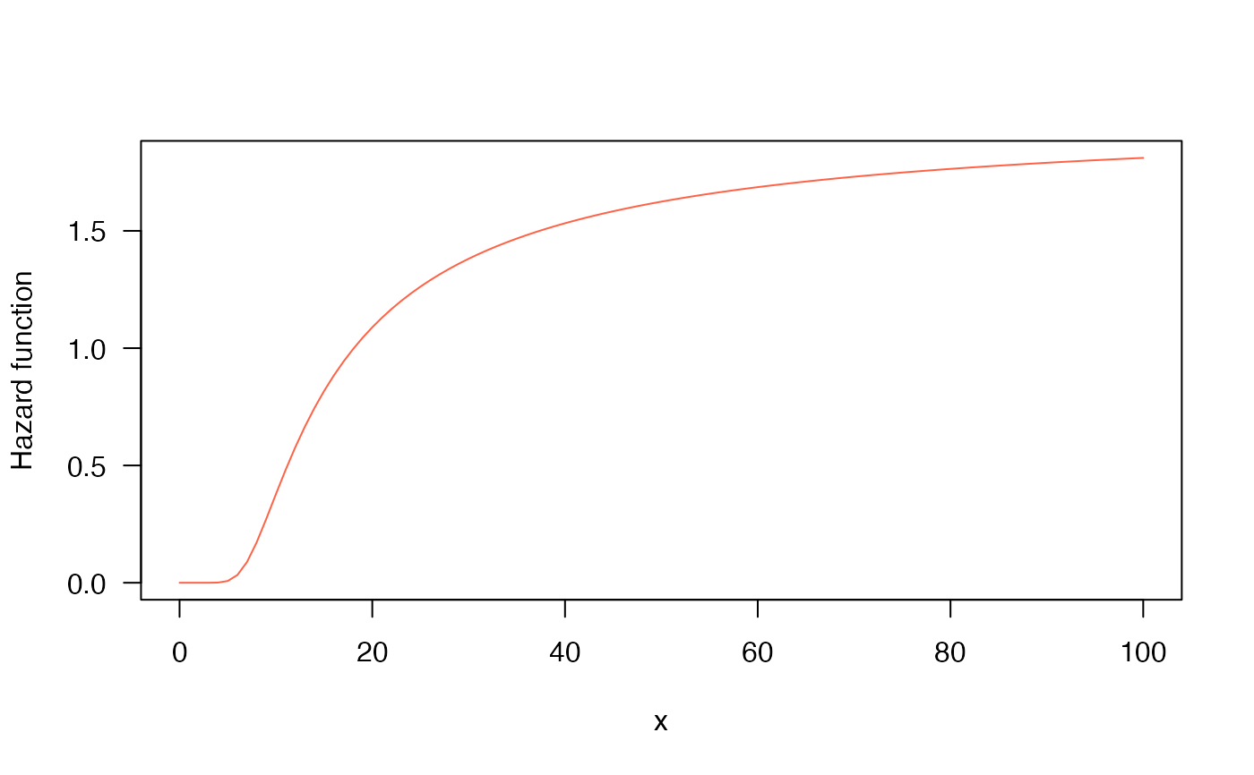
 # Example 5
# The Hazard function
curve(hGAo(x, mu=20, sigma=0.5), from=0.001, to=100,
col="tomato", ylab="Hazard function", las=1)
# Example 5
# The Hazard function
curve(hGAo(x, mu=20, sigma=0.5), from=0.001, to=100,
col="tomato", ylab="Hazard function", las=1)