These functions define the density, distribution function, quantile function and random generation for the Ex-Wald distribution with parameter \(\mu\), \(\sigma\) and \(\nu\).
Usage
dExWALD(x, mu = 1.5, sigma = 1.5, nu = 2, log = FALSE)

pExWALD(q, mu = 1.5, sigma = 1.5, nu = 2, lower.tail = TRUE, log.p = FALSE)

qExWALD(p, mu = 1.5, sigma = 1.5, nu = 2)

rExWALD(n, mu = 1.5, sigma = 1.5, nu = 2)
Arguments
- x, q
vector of (non-negative integer) quantiles.
- mu
vector of the mu parameter.
- sigma
vector of the sigma parameter.
- nu
vector of the nu parameter.
- log, log.p
logical; if TRUE, probabilities p are given as log(p).
- lower.tail
logical; if TRUE (default), probabilities are P[X <= x], otherwise, P[X > x].
- p
vector of probabilities.
- n
number of random values to return.
Value
dExWALD gives the density, pExWALD gives the distribution
function, qExWALD gives the quantile function, rExWALD
generates random deviates.
Details
The Wald distribution with parameters \(\mu\), \(\sigma\) and \(\nu\) has density given by
\(f(x |\mu, \sigma, \nu) = \frac{1}{\nu} \exp(\frac{-x}{\nu} + \sigma(\mu-k)) F_W(x|k, \sigma) \, \text{for} \, k \geq 0\)
\(f(x |\mu, \sigma, \nu) = \frac{1}{\nu} \exp\left( \frac{-(\sigma-\mu)^2}{2x} \right) Re \left( w(k^\prime \sqrt{x/2} + \frac{\sigma i}{\sqrt{2x}}) \right) \, \text{for} \, k < 0\)
where \(k=\sqrt{\mu^2-\frac{2}{\nu}}\), \(k^\prime=\sqrt{\frac{2}{\nu}-\mu^2}\) and \(F_W\) corresponds to the cumulative function of the Wald distribution.
More details about those expressions can be found on page 680 from Heathcote (2004).
References
Schwarz, W. (2001). The ex-Wald distribution as a descriptive model of response times. Behavior Research Methods, Instruments, & Computers, 33, 457-469.
Heathcote, A. (2004). Fitting Wald and ex-Wald distributions to response time data: An example using functions for the S-PLUS package. Behavior Research Methods, Instruments, & Computers, 36, 678-694.
Author
Freddy Hernandez, fhernanb@unal.edu.co
Examples
# Example 1
# Plotting the mass function for different parameter values
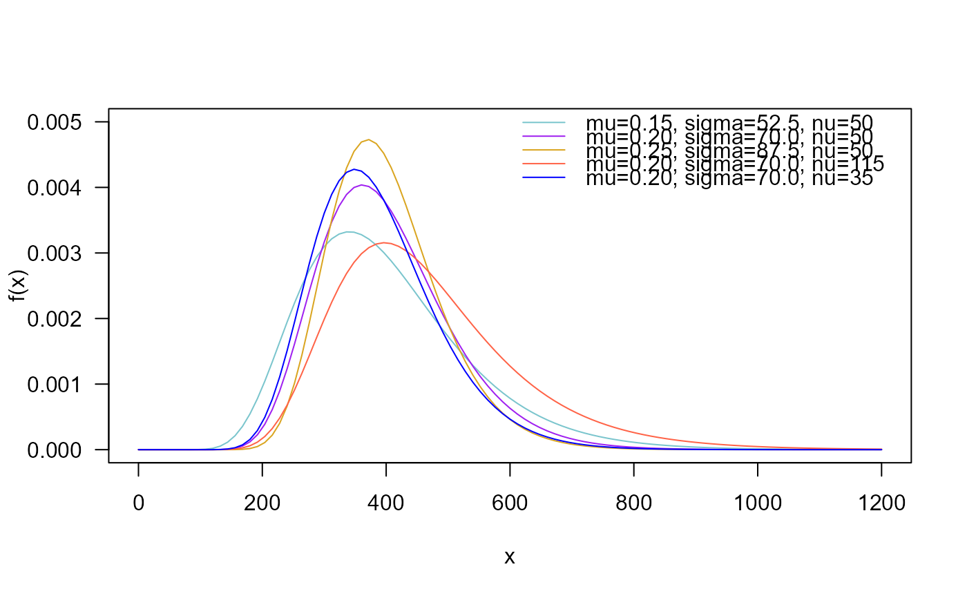
curve(dExWALD(x, mu=0.15, sigma=52.5, nu=50), ylim=c(0, 0.005),
from=0, to=1200, col="cadetblue3", las=1, ylab="f(x)")
curve(dExWALD(x, mu=0.20, sigma=70, nu=50),
add=TRUE, col= "purple")
curve(dExWALD(x, mu=0.25, sigma=87.5, nu=50),
add=TRUE, col="goldenrod")
curve(dExWALD(x, mu=0.20, sigma=70, nu=115),
add=TRUE, col="tomato")
curve(dExWALD(x, mu=0.20, sigma=70, nu=35),
add=TRUE, col="blue")
legend("topright", col=c("cadetblue3", "purple", "goldenrod",
"tomato", "blue"),
lty=1, bty="n",
legend=c("mu=0.15, sigma=52.5, nu=50",
"mu=0.20, sigma=70.0, nu=50",
"mu=0.25, sigma=87.5, nu=50",
"mu=0.20, sigma=70.0, nu=115",
"mu=0.20, sigma=70.0, nu=35"))
 # Example 2
# Checking if the cumulative curves converge to 1
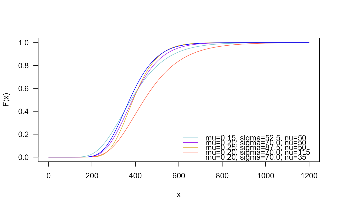
curve(pExWALD(x, mu=0.15, sigma=52.5, nu=50), ylim=c(0, 1),
from=0, to=1200, col="cadetblue3", las=1, ylab="F(x)")
curve(pExWALD(x, mu=0.20, sigma=70, nu=50),
add=TRUE, col= "purple")
curve(pExWALD(x, mu=0.25, sigma=87.5, nu=50),
add=TRUE, col="goldenrod")
curve(pExWALD(x, mu=0.20, sigma=70, nu=115),
add=TRUE, col="tomato")
curve(pExWALD(x, mu=0.20, sigma=70, nu=35),
add=TRUE, col="blue")
legend("bottomright", col=c("cadetblue3", "purple", "goldenrod",
"tomato", "blue"),
lty=1, bty="n",
legend=c("mu=0.15, sigma=52.5, nu=50",
"mu=0.20, sigma=70.0, nu=50",
"mu=0.25, sigma=87.5, nu=50",
"mu=0.20, sigma=70.0, nu=115",
"mu=0.20, sigma=70.0, nu=35"))
# Example 2
# Checking if the cumulative curves converge to 1
curve(pExWALD(x, mu=0.15, sigma=52.5, nu=50), ylim=c(0, 1),
from=0, to=1200, col="cadetblue3", las=1, ylab="F(x)")
curve(pExWALD(x, mu=0.20, sigma=70, nu=50),
add=TRUE, col= "purple")
curve(pExWALD(x, mu=0.25, sigma=87.5, nu=50),
add=TRUE, col="goldenrod")
curve(pExWALD(x, mu=0.20, sigma=70, nu=115),
add=TRUE, col="tomato")
curve(pExWALD(x, mu=0.20, sigma=70, nu=35),
add=TRUE, col="blue")
legend("bottomright", col=c("cadetblue3", "purple", "goldenrod",
"tomato", "blue"),
lty=1, bty="n",
legend=c("mu=0.15, sigma=52.5, nu=50",
"mu=0.20, sigma=70.0, nu=50",
"mu=0.25, sigma=87.5, nu=50",
"mu=0.20, sigma=70.0, nu=115",
"mu=0.20, sigma=70.0, nu=35"))
 # Example 3
# Checking the quantile function
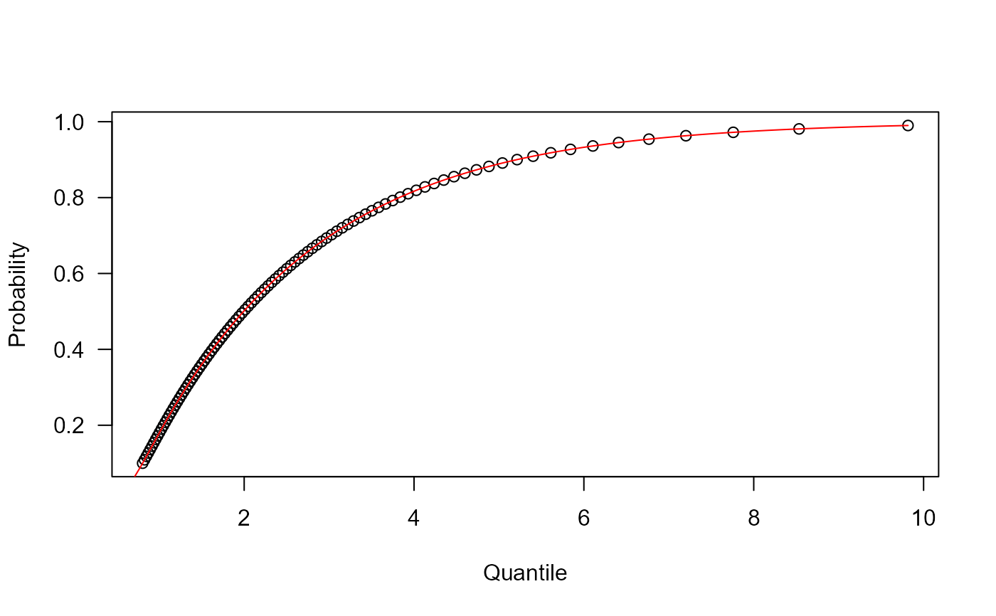
mu <- 5
sigma <- 3
nu <- 2
p <- seq(from=0.1, to=0.99, length.out=100)
plot(x=qExWALD(p, mu=mu, sigma=sigma, nu=nu), y=p, xlab="Quantile",
las=1, ylab="Probability")
curve(pExWALD(x, mu=mu, sigma=sigma, nu=nu), from=0, add=TRUE, col="red")
# Example 3
# Checking the quantile function
mu <- 5
sigma <- 3
nu <- 2
p <- seq(from=0.1, to=0.99, length.out=100)
plot(x=qExWALD(p, mu=mu, sigma=sigma, nu=nu), y=p, xlab="Quantile",
las=1, ylab="Probability")
curve(pExWALD(x, mu=mu, sigma=sigma, nu=nu), from=0, add=TRUE, col="red")
 # Example 4
# Comparing the random generator output with
# the theoretical probabilities
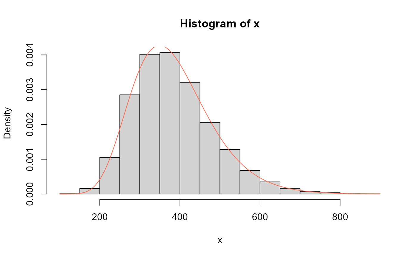
mu <- 0.2
sigma <- 70
nu <- 35
x <- rExWALD(n=10000, mu=mu, sigma=sigma, nu=nu)
hist(x, freq=FALSE)
curve(dExWALD(x, mu=mu, sigma=sigma, nu=nu), col="tomato", add=TRUE)
# Example 4
# Comparing the random generator output with
# the theoretical probabilities
mu <- 0.2
sigma <- 70
nu <- 35
x <- rExWALD(n=10000, mu=mu, sigma=sigma, nu=nu)
hist(x, freq=FALSE)
curve(dExWALD(x, mu=mu, sigma=sigma, nu=nu), col="tomato", add=TRUE)