The Exponentiated Weibull distribution

Density, distribution function, quantile function, random generation and hazard function for the exponentiated Weibull distribution with parameters mu, sigma and nu.

Usage

dEW(x, mu, sigma, nu, log = FALSE)

pEW(q, mu, sigma, nu, lower.tail = TRUE, log.p = FALSE)

qEW(p, mu, sigma, nu, lower.tail = TRUE, log.p = FALSE)

rEW(n, mu, sigma, nu)

hEW(x, mu, sigma, nu)

Arguments

x, q

vector of quantiles.

mu

scale parameter.

sigma, nu

shape parameters.

log, log.p

logical; if TRUE, probabilities p are given as log(p).

lower.tail

logical; if TRUE (default), probabilities are P[X <= x], otherwise, P[X > x].

p

vector of probabilities.

n

number of observations.

Value

dEW gives the density, pEW gives the distribution function, qEW gives the quantile function, rEW generates random deviates and hEW gives the hazard function.

Details

The Exponentiated Weibull Distribution with parameters mu, sigma and nu has density given by

\(f(x)=\nu \mu \sigma x^{\sigma-1} \exp(-\mu x^\sigma) (1-\exp(-\mu x^\sigma))^{\nu-1},\)

for \(x > 0\), \(\mu > 0\), \(\sigma > 0\) and \(\nu > 0\).

See also

EW

Examples

old_par <- par(mfrow = c(1, 1)) # save previous graphical parameters

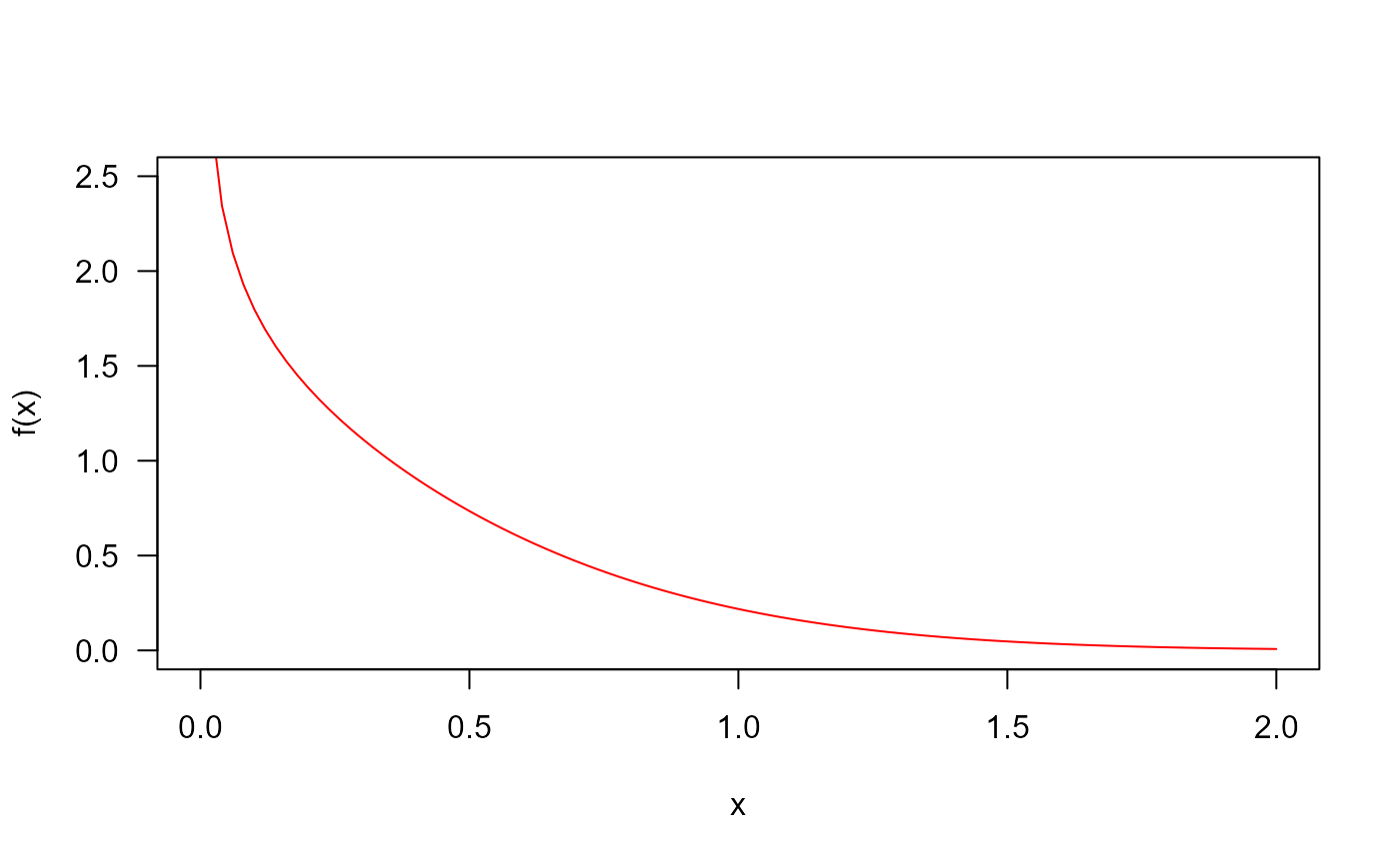
## The probability density function
curve(dEW(x, mu=2, sigma=1.5, nu=0.5), from=0, to=2,
      ylim=c(0, 2.5), col="red", las=1, ylab="f(x)") 


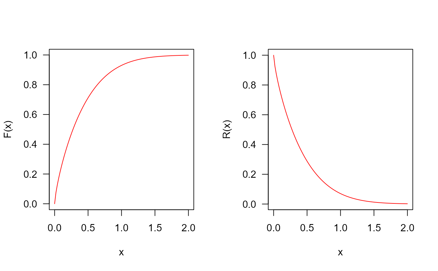
## The cumulative distribution and the Reliability function
par(mfrow=c(1, 2))
curve(pEW(x, mu=2, sigma=1.5, nu=0.5), 
      from=0, to=2,  col="red", las=1, ylab="F(x)")
curve(pEW(x, mu=2, sigma=1.5, nu=0.5, lower.tail=FALSE), 
      from=0, to=2, col="red", las=1, ylab="R(x)")


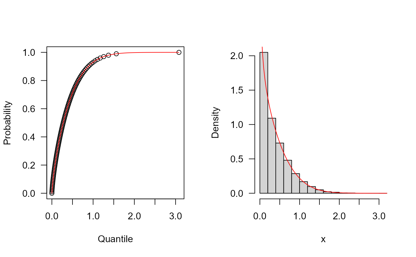
## The quantile function
p <- seq(from=0, to=0.99999, length.out=100)
plot(x=qEW(p, mu=2, sigma=1.5, nu=0.5), y=p, xlab="Quantile",
     las=1, ylab="Probability")
curve(pEW(x, mu=2, sigma=1.5, nu=0.5), from=0, add=TRUE, col="red")

## The random function
hist(rEW(n=10000, mu=2, sigma=1.5, nu=0.5), freq=FALSE, 
     xlab="x", las=1, main="")
curve(dEW(x, mu=2, sigma=1.5, nu=0.5), from=0, add=TRUE, col="red") 


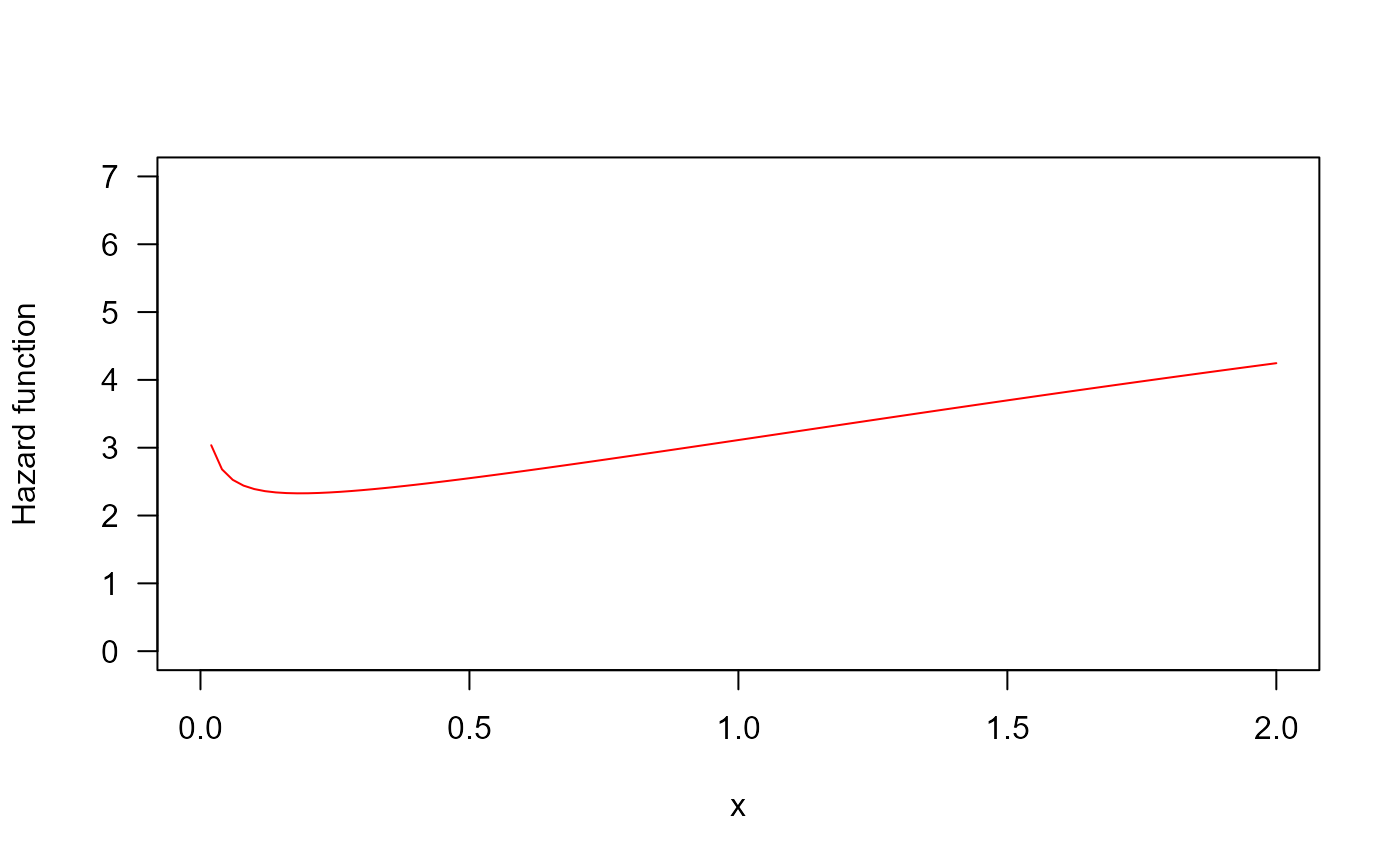
## The Hazard function
par(mfrow=c(1,1))
curve(hEW(x, mu=2, sigma=1.5, nu=0.5), from=0, to=2, ylim=c(0, 7), 
      col="red", ylab="Hazard function", las=1)


par(old_par) # restore previous graphical parameters