Density, distribution function, quantile function,
random generation and hazard function for the two-parameter
Chris-Jerry distribution with
parameters mu and sigma.
Usage
dCJ2(x, mu, sigma, log = FALSE)

pCJ2(q, mu, sigma, log.p = FALSE, lower.tail = TRUE)

qCJ2(p, mu, sigma, lower.tail = TRUE, log.p = FALSE)

rCJ2(n, mu, sigma)

hCJ2(x, mu, sigma, log = FALSE)Value
dCJ2 gives the density, pCJ2 gives the distribution
function, qCJ2 gives the quantile function, rCJ2
generates random deviates and hCJ2 gives the hazard function.
Details
The two-parameter Chris-Jerry distribution with parameters mu
and sigma has density given by
\( f(x; \sigma, \mu) = \frac{\mu^2}{\sigma \mu + 2} (\sigma + \mu x^2) e^{-\mu x}; \quad x > 0, \quad \mu > 0, \quad \sigma > 0 \)
Note: In this implementation we changed the original parameters \(\theta\) for \(\mu\) and \(\lambda\) for \(\sigma\), we did it to implement this distribution within gamlss framework.
References
Chinedu, Eberechukwu Q., et al. "New lifetime distribution with applications to single acceptance sampling plan and scenarios of increasing hazard rates" Symmetry 15.10 (2023): 188.
Author
Manuel Gutierrez Tangarife, mgutierrezta@unal.edu.co
Examples
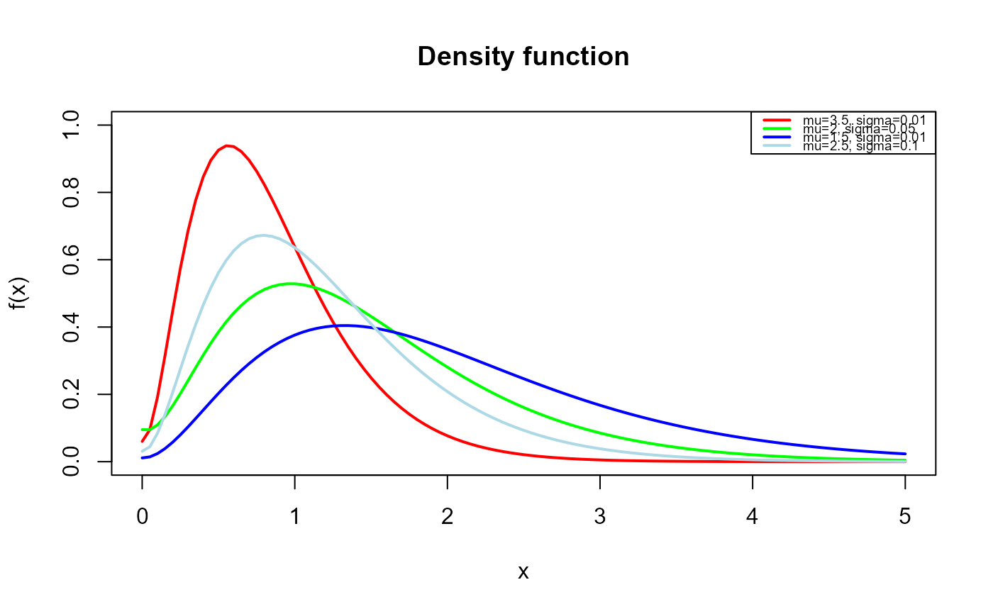
# Example 1
# Plotting the density function for different parameter values
curve(dCJ2(x, mu=3.5, sigma=0.01),
from=0.0001, to=5,
ylim=c(0, 1),
col="red", lwd=2,
main="Density function",
xlab="x", ylab="f(x)")
curve(dCJ2(x, mu=2, sigma=0.05),
col="green",
lwd=2,
add=TRUE)
curve(dCJ2(x, mu=1.5, sigma=0.01),
col="blue",
lwd=2,
add=TRUE)
curve(dCJ2(x, mu=2.5, sigma=0.01),
col="lightblue",
lwd=2,
add=TRUE)
legend("topright", legend=c("mu=3.5, sigma=0.01",
"mu=2, sigma=0.05",
"mu=1.5, sigma=0.01",
"mu=2.5, sigma=0.1"),
col=c( "red", "green","blue","lightblue"), lwd=2, cex=0.6)
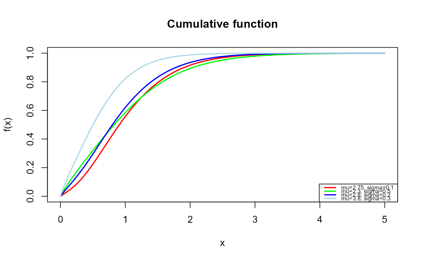
 # Example 2
# Checking if the cumulative curves converge to 1
curve(pCJ2(x, mu=2.7, sigma=0.1),
from=0.0001, to=5,
ylim=c(0, 1),
col="red", lwd=2,
main="Cumulative function",
xlab="x", ylab="f(x)")
curve(pCJ2(x, mu=2.3, sigma=0.5),
col="green",
lwd=2,
add=TRUE)
curve(pCJ2(x, mu=2.8, sigma=0.2),
col="blue",
lwd=2,
add=TRUE)
curve(pCJ2(x, mu=3.8, sigma=0.3),
col="lightblue",
lwd=2,
add=TRUE)
legend("bottomright", legend=c("mu=2.75, sigma=0.1",
"mu=2.3, sigma=0.5",
"mu=2.8, sigma=0.2",
"mu=3.8, sigma=0.3"),
col=c( "red", "green","blue","lightblue"), lwd=2, cex=0.6)
# Example 2
# Checking if the cumulative curves converge to 1
curve(pCJ2(x, mu=2.7, sigma=0.1),
from=0.0001, to=5,
ylim=c(0, 1),
col="red", lwd=2,
main="Cumulative function",
xlab="x", ylab="f(x)")
curve(pCJ2(x, mu=2.3, sigma=0.5),
col="green",
lwd=2,
add=TRUE)
curve(pCJ2(x, mu=2.8, sigma=0.2),
col="blue",
lwd=2,
add=TRUE)
curve(pCJ2(x, mu=3.8, sigma=0.3),
col="lightblue",
lwd=2,
add=TRUE)
legend("bottomright", legend=c("mu=2.75, sigma=0.1",
"mu=2.3, sigma=0.5",
"mu=2.8, sigma=0.2",
"mu=3.8, sigma=0.3"),
col=c( "red", "green","blue","lightblue"), lwd=2, cex=0.6)
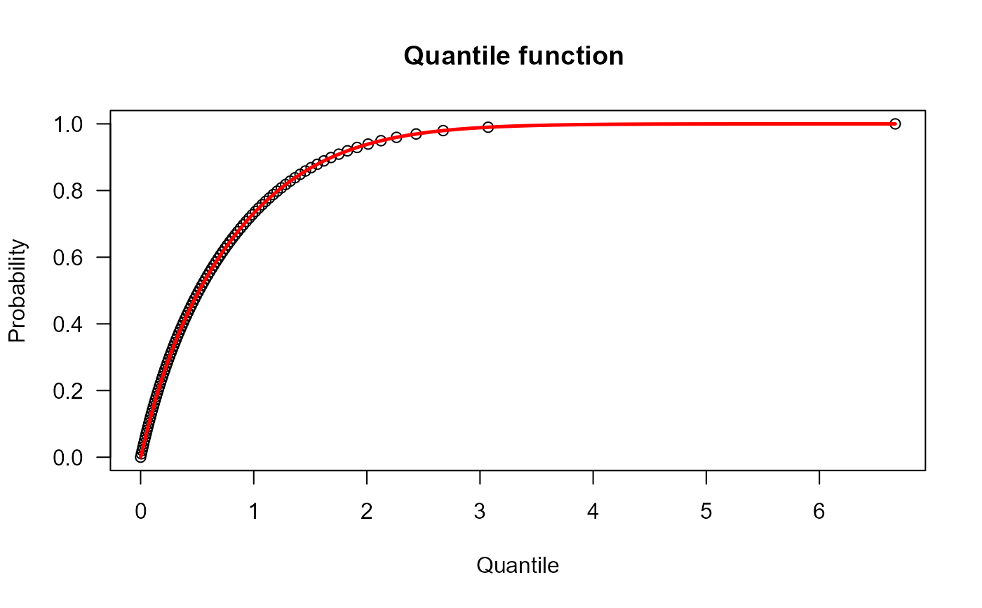
 # Example 3
# Checking the quantile function
p <- seq(from=0.0001, to=0.99999, length.out=100)
plot(x=qCJ2(p, mu=2.3, sigma=1.7), y=p, xlab="Quantile",
las=1, ylab="Probability", main="Quantile function ")
curve(pCJ2(x, mu=2.3, sigma=1.7),
from=0.0001, add=TRUE, col="red", lwd=2.5)
# Example 3
# Checking the quantile function
p <- seq(from=0.0001, to=0.99999, length.out=100)
plot(x=qCJ2(p, mu=2.3, sigma=1.7), y=p, xlab="Quantile",
las=1, ylab="Probability", main="Quantile function ")
curve(pCJ2(x, mu=2.3, sigma=1.7),
from=0.0001, add=TRUE, col="red", lwd=2.5)
 # Example 4
# Comparing the random generator output with
# the theoretical probabilities
x <- rCJ2(n=10000, mu=1.5, sigma=2.5)
hist(x, freq=FALSE)
curve(dCJ2(x, mu=1.5, sigma=2.5), from=0.001, to=8,
add=TRUE, col="tomato", lwd=2)
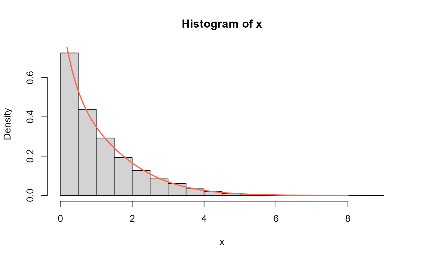
# Example 4
# Comparing the random generator output with
# the theoretical probabilities
x <- rCJ2(n=10000, mu=1.5, sigma=2.5)
hist(x, freq=FALSE)
curve(dCJ2(x, mu=1.5, sigma=2.5), from=0.001, to=8,
add=TRUE, col="tomato", lwd=2)
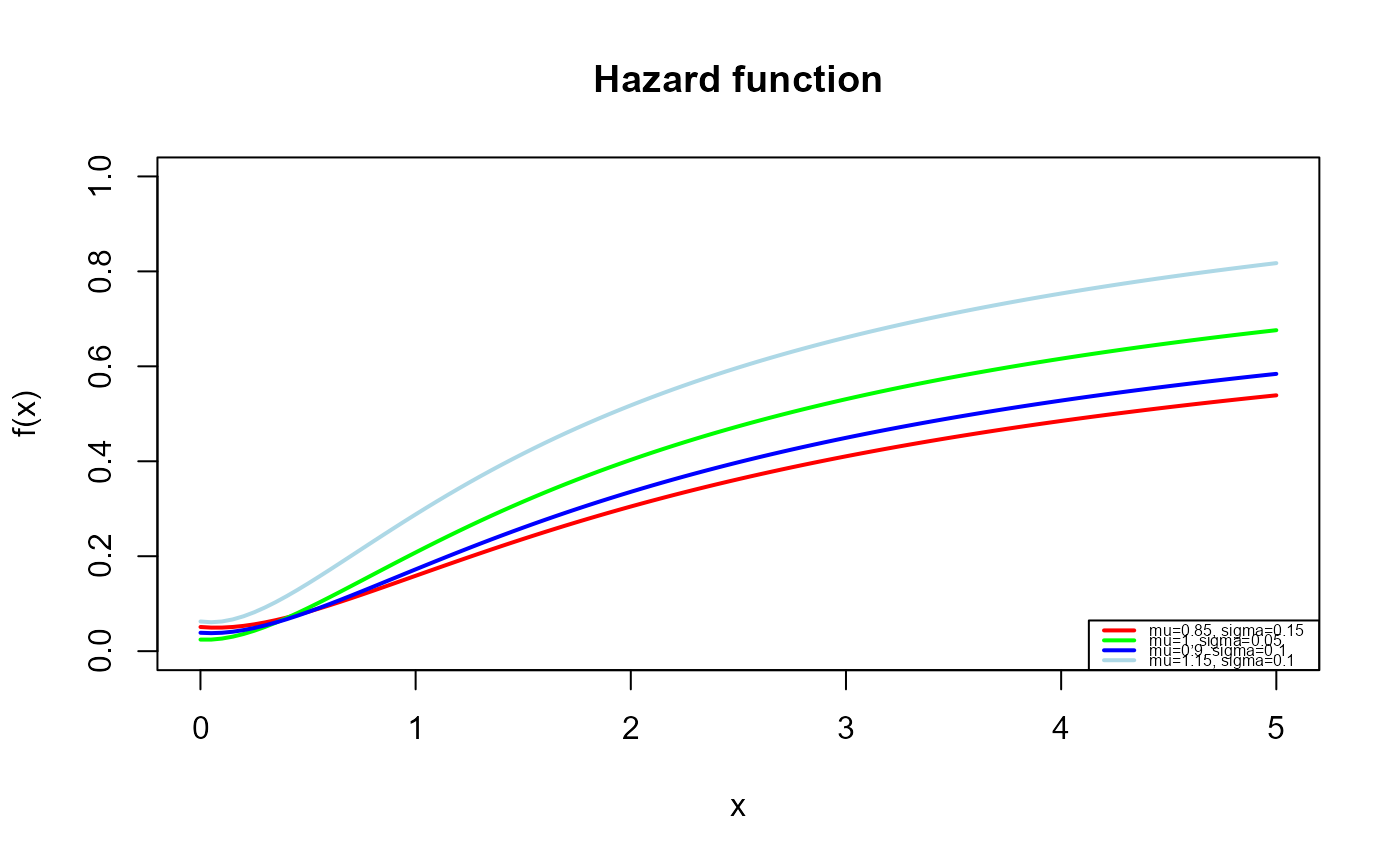
 # Example 5
# The Hazard function
curve(hCJ2(x, mu=0.85, sigma=0.15),
from=0.0001, to=5,
ylim=c(0, 1),
col="red", lwd=2,
main="Hazard function",
xlab="x", ylab="f(x)")
curve(hCJ2(x, mu=1, sigma=0.05),
col="green",
lwd=2,
add=TRUE)
curve(hCJ2(x, mu=0.9, sigma=0.1),
col="blue",
lwd=2,
add=TRUE)
curve(hCJ2(x, mu=1.15, sigma=0.1),
col="lightblue",
lwd=2,
add=TRUE)
legend("bottomright", legend=c("mu=0.85, sigma=0.15",
"mu=1, sigma=0.05",
"mu=0.9, sigma=0.1",
"mu=1.15, sigma=0.1"),
col=c( "red", "green","blue","lightblue"), lwd=2, cex=0.5)
# Example 5
# The Hazard function
curve(hCJ2(x, mu=0.85, sigma=0.15),
from=0.0001, to=5,
ylim=c(0, 1),
col="red", lwd=2,
main="Hazard function",
xlab="x", ylab="f(x)")
curve(hCJ2(x, mu=1, sigma=0.05),
col="green",
lwd=2,
add=TRUE)
curve(hCJ2(x, mu=0.9, sigma=0.1),
col="blue",
lwd=2,
add=TRUE)
curve(hCJ2(x, mu=1.15, sigma=0.1),
col="lightblue",
lwd=2,
add=TRUE)
legend("bottomright", legend=c("mu=0.85, sigma=0.15",
"mu=1, sigma=0.05",
"mu=0.9, sigma=0.1",
"mu=1.15, sigma=0.1"),
col=c( "red", "green","blue","lightblue"), lwd=2, cex=0.5)