The Beta Transformed Lomax distribution

Density, distribution function, quantile function and random generation for the Beta Transformed Lomax distribution with parameters mu, sigma and nu.

Usage

dBTL(x, mu = 1.5, sigma = 1.5, nu = 2, log = FALSE)

pBTL(q, mu = 1.5, sigma = 1.5, nu = 2, lower.tail = TRUE, log.p = FALSE)

qBTL(p, mu = 1.5, sigma = 1.5, nu = 2, lower.tail = TRUE, log.p = FALSE)

rBTL(n, mu = 1.5, sigma = 1.5, nu = 2)

Arguments

x, q: vector of quantiles.
mu: parameter.
sigma: parameter.
nu: parameter.
log, log.p: logical; if TRUE, probabilities p are given as log(p).
lower.tail: logical; if TRUE (default), probabilities are P[X <= x], otherwise, P[X > x].
p: vector of probabilities.
n: number of observations.

Value

dBTL gives the density, pBTL gives the distribution function, qBTL gives the quantile function and rBTL generates random deviates.

Details

The Beta Transformed Lomax distribution with parameters mu, sigma and nu has density given by

\(f(x) = \frac{\log \nu}{\nu-1} \frac{\sigma}{\mu} \left(1+\frac{x}{\mu}\right)^{-(\sigma+1)} \nu^{\left(1+\frac{x}{\mu}\right)^{-\sigma}},\)

for \(\nu \neq 1\), and for \(\nu = 1\):

\(f(x) = \frac{\sigma}{\mu} \left(1+\frac{x}{\mu}\right)^{-(\sigma+1)},\)

for \(x \geq 0\), \(\mu > 0\), \(\sigma > 0\) and \(\nu > 0\).

References

Kottakkunnan, F. A New Generalization of Lomax Distribution: Estimation and Modelling for Medical Data. J Stat Theory Appl 25, 19 (2026). https://doi.org/10.1007/s44199-026-00171-0

Author

Marieth Guillen, mguillen@unal.edu.co

Examples

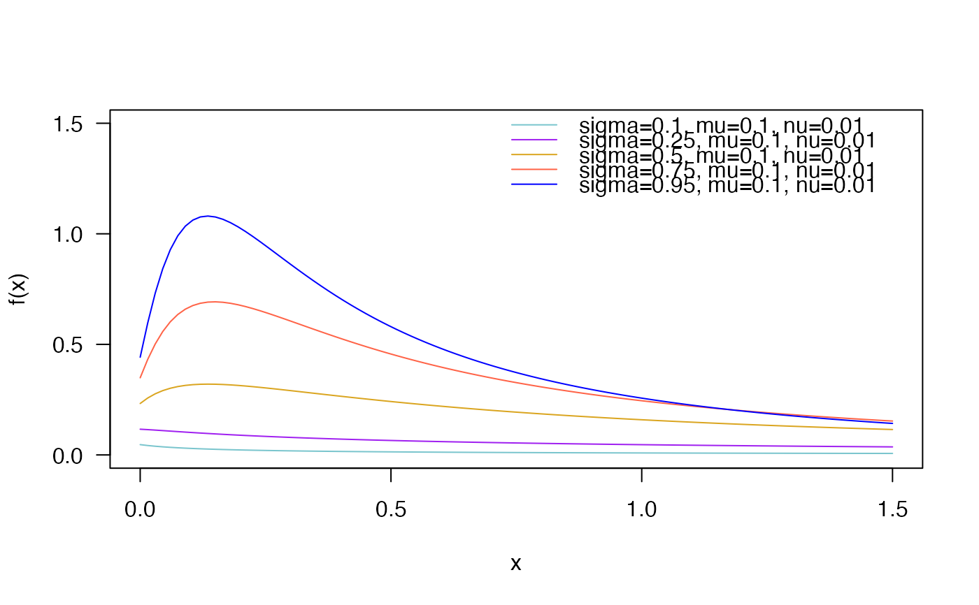
# Example 1
# Plotting the density function for different parameter values
curve(dBTL(x, sigma=0.1, mu=0.1, nu=0.01),
      ylim=c(0, 1.5),
      from=0, to=1.5, col="cadetblue3",
      las=1, ylab="f(x)")
curve(dBTL(x, sigma=0.25, mu=0.1, nu=0.01),
      add=TRUE, col= "purple")
curve(dBTL(x, sigma=0.5, mu=0.1, nu=0.01),
      add=TRUE, col="goldenrod")
curve(dBTL(x, sigma=0.75, mu=0.1, nu=0.01),
      add=TRUE, col="tomato")
curve(dBTL(x, sigma=0.95, mu=0.1, nu=0.01),
      add=TRUE, col="blue")
legend("topright", col=c("cadetblue3", "purple", "goldenrod", "tomato", "blue"),
       lty=1, bty="n", legend=c("sigma=0.1, mu=0.1, nu=0.01",
                                "sigma=0.25, mu=0.1, nu=0.01",
                                "sigma=0.5, mu=0.1, nu=0.01",
                                "sigma=0.75, mu=0.1, nu=0.01",
                                "sigma=0.95, mu=0.1, nu=0.01"))


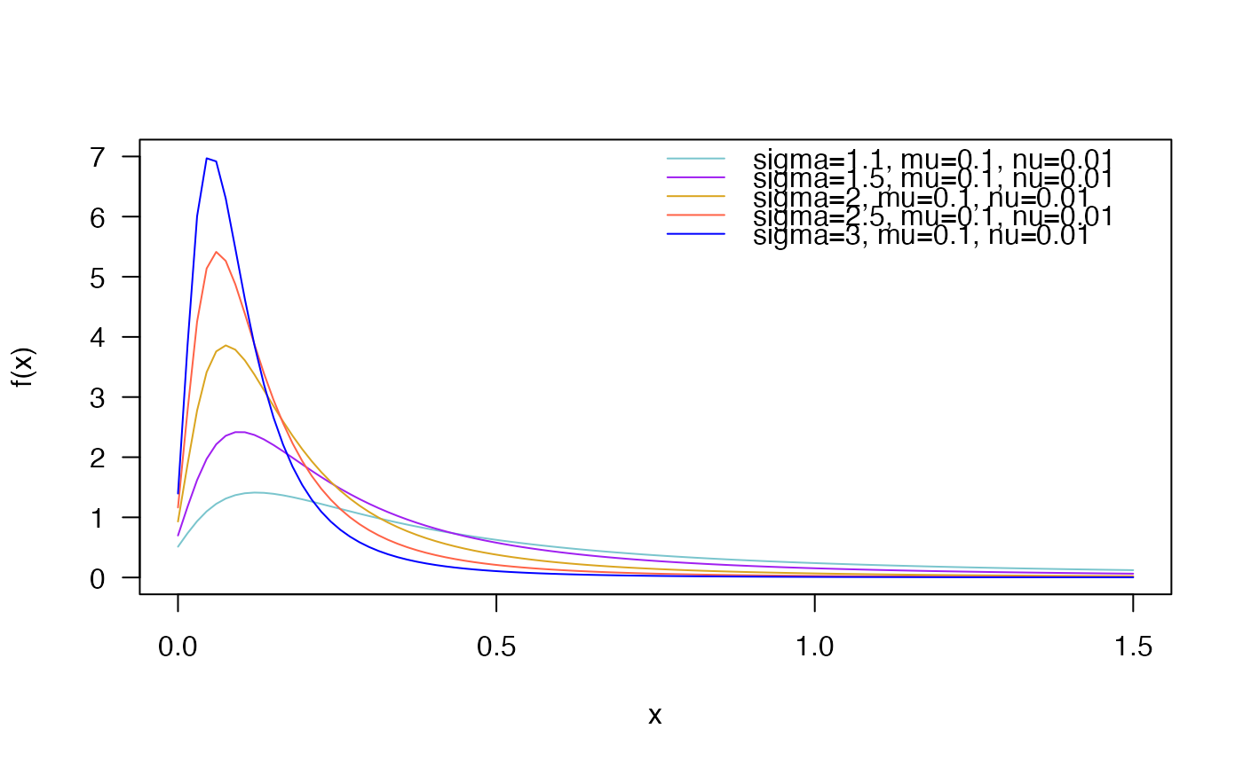
curve(dBTL(x, sigma=1.1, mu=0.1, nu=0.01),
      ylim=c(0, 7),
      from=0, to=1.5, col="cadetblue3",
      las=1, ylab="f(x)")
curve(dBTL(x, sigma=1.5, mu=0.1, nu=0.01),
      add=TRUE, col= "purple")
curve(dBTL(x, sigma=2, mu=0.1, nu=0.01),
      add=TRUE, col="goldenrod")
curve(dBTL(x, sigma=2.5, mu=0.1, nu=0.01),
      add=TRUE, col="tomato")
curve(dBTL(x, sigma=3, mu=0.1, nu=0.01),
      add=TRUE, col="blue")
legend("topright", col=c("cadetblue3", "purple", "goldenrod", "tomato", "blue"),
       lty=1, bty="n", legend=c("sigma=1.1, mu=0.1, nu=0.01",
                                "sigma=1.5, mu=0.1, nu=0.01",
                                "sigma=2, mu=0.1, nu=0.01",
                                "sigma=2.5, mu=0.1, nu=0.01",
                                "sigma=3, mu=0.1, nu=0.01"))


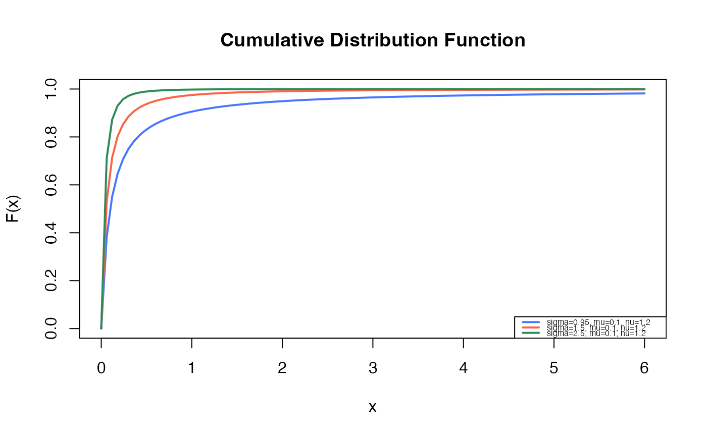
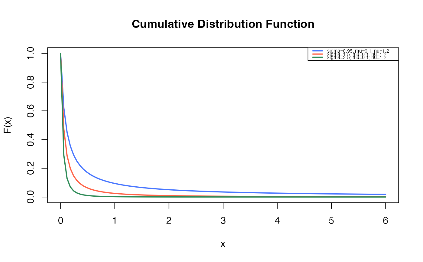
# Example 2
# Checking if the cumulative curves converge to 1
curve(pBTL(x, sigma=0.95, mu=0.1, nu=1.2),
      from=0, to=6, 
      ylim=c(0, 1),
      col="royalblue1", lwd=2,
      main="Cumulative Distribution Function",
      xlab="x", ylab="F(x)")
curve(pBTL(x, sigma=1.5, mu=0.1, nu=1.2),
      col="tomato",
      lwd=2,
      add=TRUE)
curve(pBTL(x, sigma=2.5, mu=0.1, nu=1.2),
      col="seagreen",
      lwd=2,
      add=TRUE)
legend("bottomright", legend=c("sigma=0.95, mu=0.1, nu=1.2",
                               "sigma=1.5, mu=0.1, nu=1.2",
                               "sigma=2.5, mu=0.1, nu=1.2"),
       col=c("royalblue1", "tomato", "seagreen"), lwd=2, cex=0.5)


curve(pBTL(x, sigma=0.95, mu=0.1, nu=1.2, lower.tail=FALSE),
      from=0, to=6, 
      ylim=c(0, 1),
      col="royalblue1", lwd=2,
      main="Cumulative Distribution Function",
      xlab="x", ylab="F(x)")
curve(pBTL(x, sigma=1.5, mu=0.1, nu=1.2, lower.tail=FALSE),
      col="tomato",
      lwd=2,
      add=TRUE)
curve(pBTL(x, sigma=2.5, mu=0.1, nu=1.2, lower.tail=FALSE),
      col="seagreen",
      lwd=2,
      add=TRUE)
legend("topright", legend=c("sigma=0.95, mu=0.1, nu=1.2",
                            "sigma=1.5, mu=0.1, nu=1.2",
                            "sigma=2.5, mu=0.1, nu=1.2"),
       col=c("royalblue1", "tomato", "seagreen"), lwd=2, cex=0.5)


# Example 3
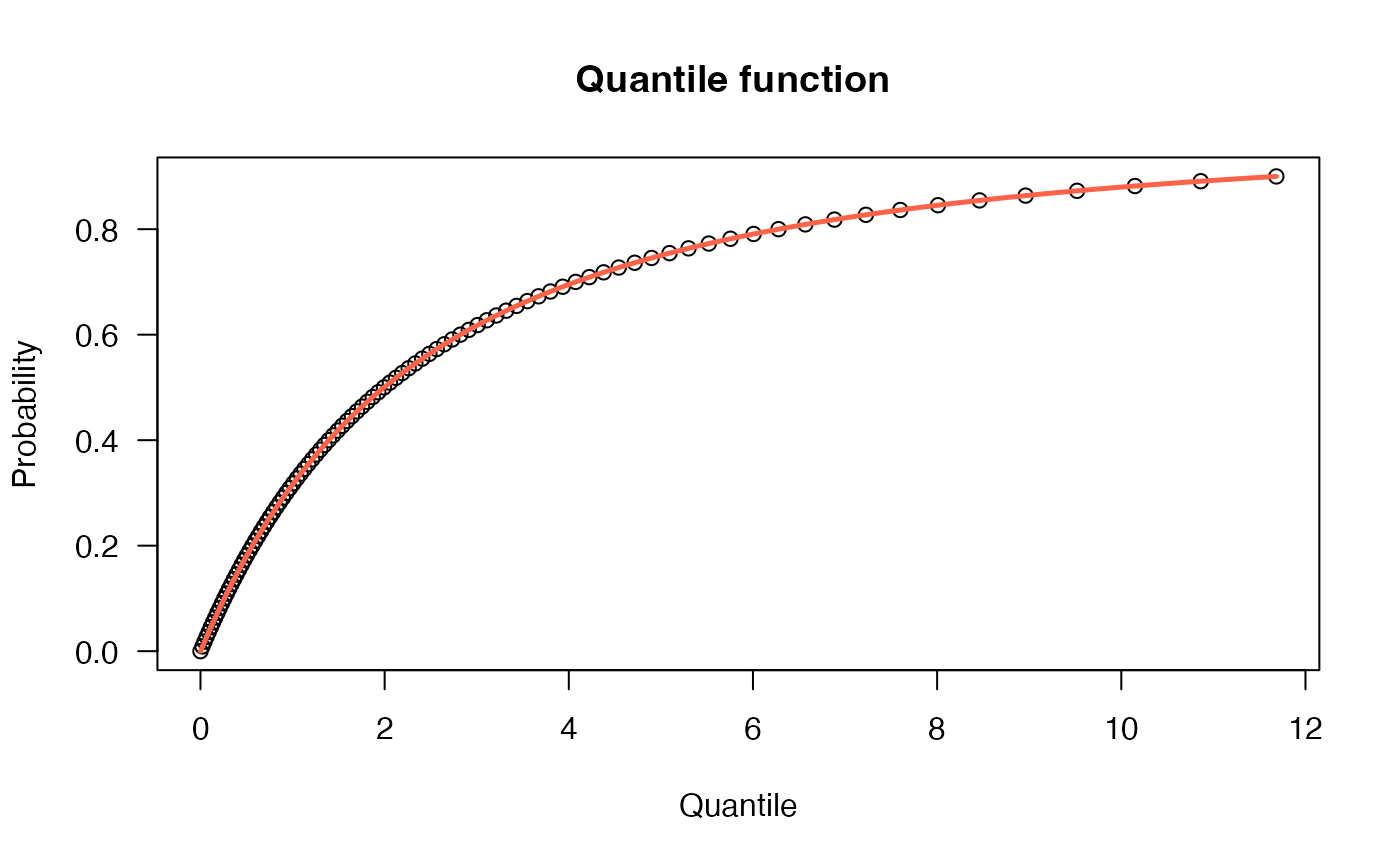
# The quantile function
p <- seq(from=0, to=0.9, length.out=100)
plot(x=qBTL(p, mu=2.5, sigma=1.5, nu=0.5), y=p, xlab="Quantile",
     las=1, ylab="Probability", main="Quantile function ")
curve(pBTL(q=x, mu=2.5, sigma=1.5, nu=0.5),
      from=0, add=TRUE, col="tomato", lwd=2.5)


# Example 4
# The random function
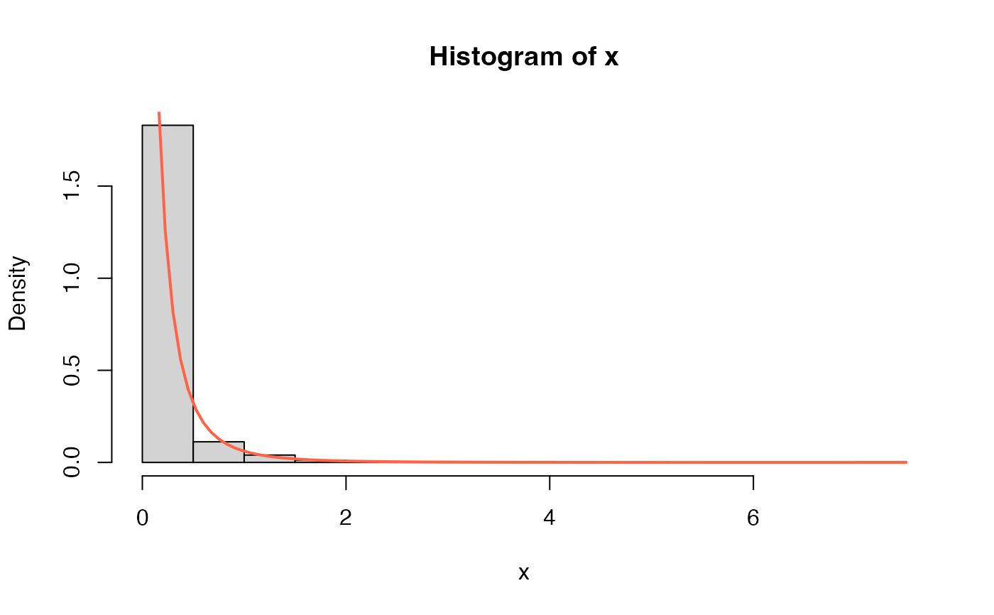
x <- rBTL(n=1000, mu=0.5, sigma=3, nu=1.5)
hist(x, freq=FALSE)
curve(dBTL(x, mu=0.5, sigma=3, nu=1.5), from=0, 
      add=TRUE, col="tomato", lwd=2)