The Birnbaum-Saunders distribution - Santos-Neto et al. (2012) (P7 based on the mean and a bounded variance)
Source:R/dBS9.R
dBS9.RdDensity, distribution function, quantile function,
random generation and hazard function for the
Birnbaum-Saunders distribution with
parameters mu and sigma.
Usage
dBS9(x, mu = 0.5, sigma = 10, log = FALSE)

pBS9(q, mu = 1, sigma = 2, lower.tail = TRUE, log.p = FALSE)

qBS9(p, mu = 1, sigma = 2, lower.tail = TRUE, log.p = FALSE)

rBS9(n, mu = 1, sigma = 2)

hBS9(x, mu, sigma)
Arguments
- x, q
vector of quantiles.
- mu
parameter representing the shape (
mu > 0).- sigma
parameter representing the variance (
sigma > 0).- log, log.p
logical; if TRUE, probabilities p are given as log(p).
- lower.tail
logical; if TRUE (default), probabilities are P[X <= x], otherwise, P[X > x].
- p
vector of probabilities.
- n
number of observations.
Value
dBS9 gives the density, pBS9 gives the distribution
function, qBS9 gives the quantile function, rBS9
generates random deviates and hBS9 gives the hazard function.
Details
The Birnbaum-Saunders with parameters mu and sigma
has density given by
$$ f(x \mid \mu,\sigma) = \frac{ \exp\left(\frac{1}{2(\sigma-1)}\right) (x\sigma+\mu) }{ 4\sqrt{\pi\sigma(\sigma-1)\mu}\,x^{3/2} } \exp\left[ -\frac{1}{4(\sigma-1)} \left( \frac{x\sigma}{\mu}+ \frac{\mu}{x\sigma} \right) \right] $$
for \(x>0\), \(\mu>0\) and \(\sigma>1\). In this parameterization, \(E(X) = \mu\) and \(Var(X) = \frac{\mu^2(\sigma-1)(5\sigma-3)}{\sigma^2}\).
References
Santos-Neto, M., Cysneiros, F. J. A., Leiva, V., & Ahmed, S. E. (2012). On new parameterizations of the Birnbaum-Saunders distribution. Pakistan Journal of Statistics, 28(1), 1-26.
See also
BS9.
Author
David Villegas Ceballos, david.villegas1@udea.edu.co
Examples
# Example 1
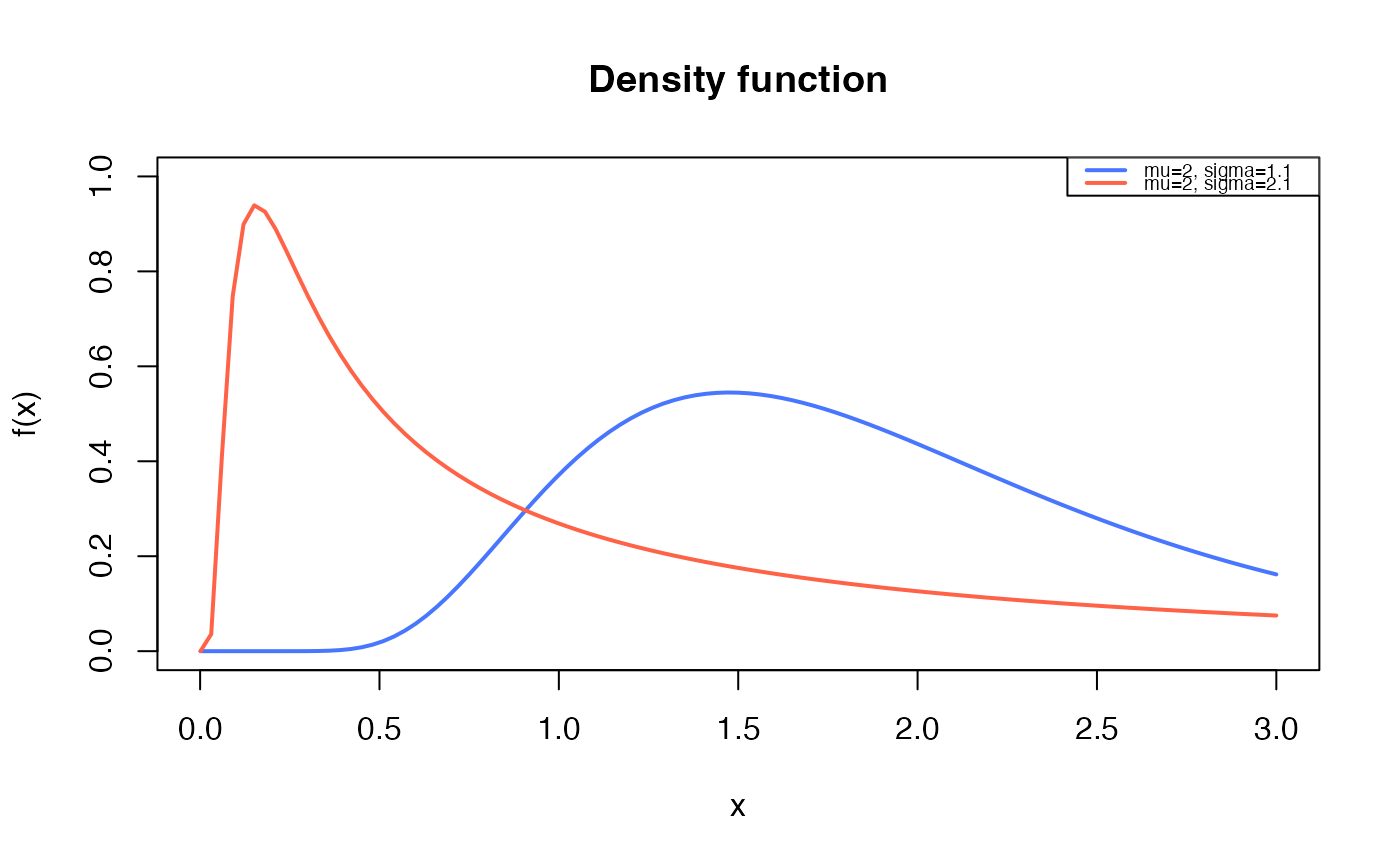
# Plotting the mass function for different parameter values
curve(dBS9(x, mu=2, sigma=1.1),
from=0.001, to=3,
ylim=c(0, 1.0),
col="royalblue1", lwd=2,
main="Density function",
xlab="x", ylab="f(x)")
curve(dBS9(x, mu=2, sigma=2.1),
col="tomato",
lwd=2,
add=TRUE)
legend("topright", legend=c("mu=2, sigma=1.1",
"mu=2, sigma=2.1"),
col=c("royalblue1", "tomato"), lwd=2, cex=0.6)
 # Example 2
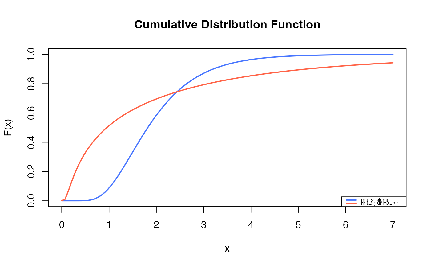
# Checking if the cumulative curves converge to 1
curve(pBS9(x, mu=2, sigma=1.1),
from=0.00001, to=7,
ylim=c(0, 1),
col="royalblue1", lwd=2,
main="Cumulative Distribution Function",
xlab="x", ylab="F(x)")
curve(pBS9(x, mu=2, sigma=2.1),
col="tomato",
lwd=2,
add=TRUE)
legend("bottomright", legend=c("mu=2, sigma=1.1",
"mu=2, sigma=2.1"),
col=c("royalblue1", "tomato"), lwd=2, cex=0.5)
# Example 2
# Checking if the cumulative curves converge to 1
curve(pBS9(x, mu=2, sigma=1.1),
from=0.00001, to=7,
ylim=c(0, 1),
col="royalblue1", lwd=2,
main="Cumulative Distribution Function",
xlab="x", ylab="F(x)")
curve(pBS9(x, mu=2, sigma=2.1),
col="tomato",
lwd=2,
add=TRUE)
legend("bottomright", legend=c("mu=2, sigma=1.1",
"mu=2, sigma=2.1"),
col=c("royalblue1", "tomato"), lwd=2, cex=0.5)
 # Example 3
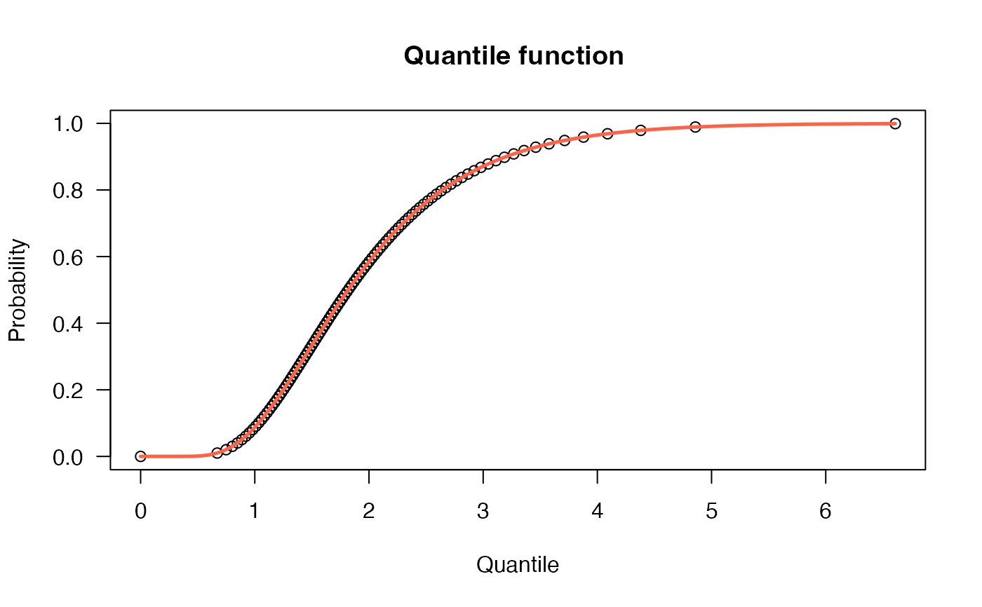
# The quantile function
p <- seq(from=0, to=0.999, length.out=100)
plot(x=qBS9(p, mu=2, sigma=1.1), y=p, xlab="Quantile",
las=1, ylab="Probability", main="Quantile function ")
curve(pBS9(x, mu=2, sigma=1.1),
from=0, add=TRUE, col="tomato", lwd=2.5)
# Example 3
# The quantile function
p <- seq(from=0, to=0.999, length.out=100)
plot(x=qBS9(p, mu=2, sigma=1.1), y=p, xlab="Quantile",
las=1, ylab="Probability", main="Quantile function ")
curve(pBS9(x, mu=2, sigma=1.1),
from=0, add=TRUE, col="tomato", lwd=2.5)
 # Example 4
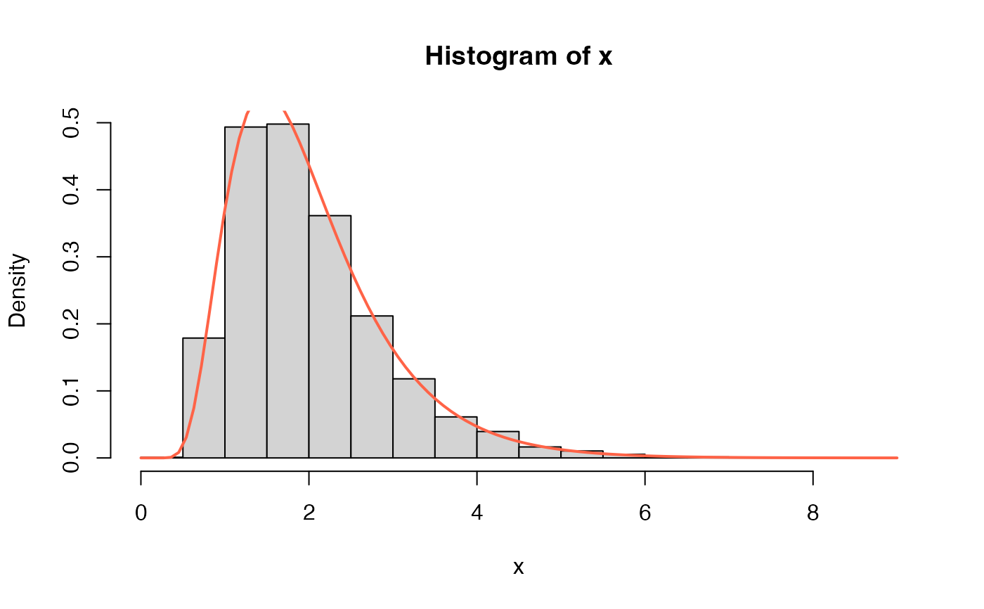
# The random function
x <- rBS9(n=10000, mu=2, sigma=1.1)
hist(x, freq=FALSE)
curve(dBS9(x, mu=2, sigma=1.1),
add=TRUE, col="tomato", lwd=2)
# Example 4
# The random function
x <- rBS9(n=10000, mu=2, sigma=1.1)
hist(x, freq=FALSE)
curve(dBS9(x, mu=2, sigma=1.1),
add=TRUE, col="tomato", lwd=2)
 # Example 5
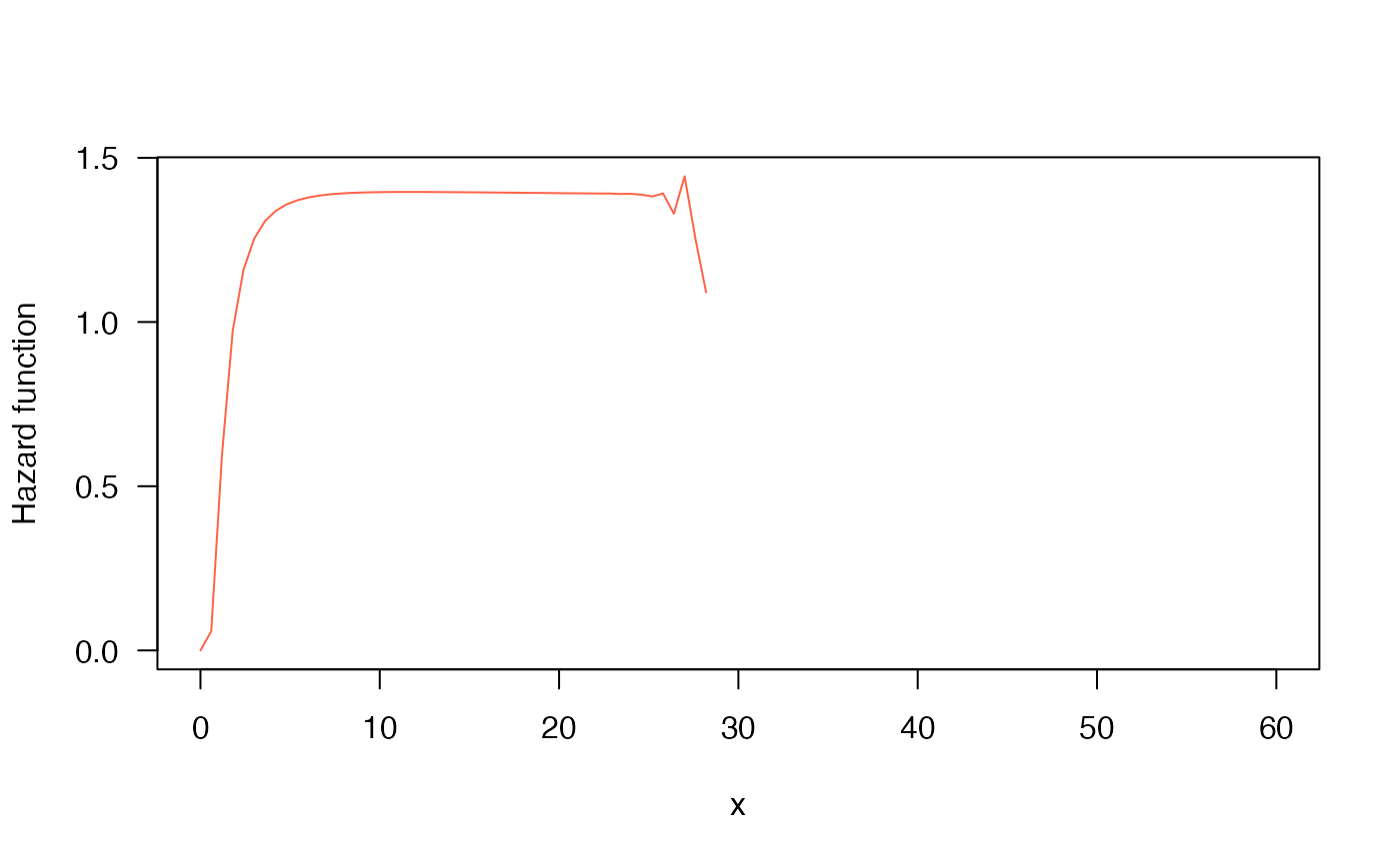
# The Hazard function
curve(hBS9(x, mu=2, sigma=1.1), from=0.001, to=60,
col="tomato", ylab="Hazard function", las=1)
# Example 5
# The Hazard function
curve(hBS9(x, mu=2, sigma=1.1), from=0.001, to=60,
col="tomato", ylab="Hazard function", las=1)