Density, distribution function, quantile function,
random generation and hazard function for the
Birnbaum-Saunders distribution with
parameters mu and sigma.
Usage
dBS4(x, mu = 1, sigma = 0.5, log = FALSE)

pBS4(q, mu = 1, sigma = 0.5, lower.tail = TRUE, log.p = FALSE)

qBS4(p, mu = 1, sigma = 0.5, lower.tail = TRUE, log.p = FALSE)

rBS4(n, mu = 1, sigma = 0.5)

hBS4(x, mu, sigma)Value
dBS4 gives the density, pBS4 gives the distribution
function, qBS4 gives the quantile function, rBS4
generates random deviates and hBS4 gives the hazard function.
Details
The Birnbaum-Saunders with parameters mu and sigma
has density given by
\(f(x|\mu,\sigma) = \frac{1}{2\sqrt{2\pi}} \left[ \frac{\sigma}{x\sqrt{x}} + \frac{\mu}{\sqrt{x}} \right] \exp\left( -\frac{1}{2} \left[ \frac{\sigma}{\sqrt{x}} - \mu\sqrt{x} \right]^2 \right)\)
for \(x>0\), \(\mu>0\) and \(\sigma>0\). In this parameterization \(E(X) = \frac{\sigma \mu + 1/2}{\mu^2}\) and \(Var(X) = \frac{\sigma \mu + 5/4}{\mu^4}\).
References
Ahmed, S. E., Budsaba, K., Lisawadi, S., & Volodin, A. (2008). Parametric estimation for the Birnbaum-Saunders lifetime distribution based on a new parametrization. Thailand Statistician, 6(2), 213-240.
See also
BS4.
Author
David Villegas Ceballos, david.villegas1@udea.edu.co
Examples
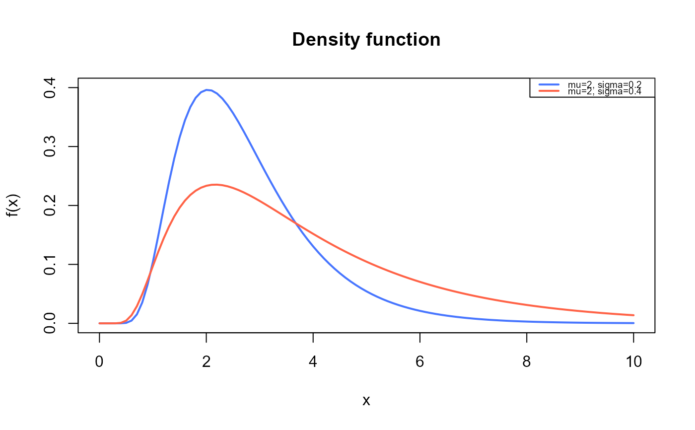
# Example 1
# Plotting the mass function for different parameter values
curve(dBS4(x, mu=2, sigma=30),
from=0.001, to=40,
ylim=c(0, 0.20),
col="royalblue1", lwd=2,
main="Density function",
xlab="x", ylab="f(x)")
curve(dBS4(x, mu=1, sigma=20),
col="tomato",
lwd=2,
add=TRUE)
legend("topright", legend=c("mu=2, sigma=30",
"mu=1, sigma=20"),
col=c("royalblue1", "tomato"), lwd=2, cex=0.6)
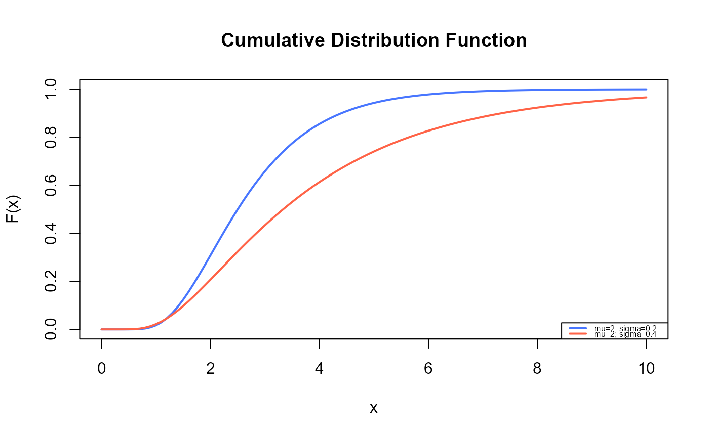
 # Example 2
# Checking if the cumulative curves converge to 1
curve(pBS4(x, mu=2, sigma=30),
from=0.00001, to=40,
ylim=c(0, 1),
col="royalblue1", lwd=2,
main="Cumulative Distribution Function",
xlab="x", ylab="F(x)")
curve(pBS4(x, mu=1, sigma=20),
col="tomato",
lwd=2,
add=TRUE)
legend("bottomright", legend=c("mu=2, sigma=30",
"mu=1, sigma=20"),
col=c("royalblue1", "tomato", "seagreen"), lwd=2, cex=0.5)
# Example 2
# Checking if the cumulative curves converge to 1
curve(pBS4(x, mu=2, sigma=30),
from=0.00001, to=40,
ylim=c(0, 1),
col="royalblue1", lwd=2,
main="Cumulative Distribution Function",
xlab="x", ylab="F(x)")
curve(pBS4(x, mu=1, sigma=20),
col="tomato",
lwd=2,
add=TRUE)
legend("bottomright", legend=c("mu=2, sigma=30",
"mu=1, sigma=20"),
col=c("royalblue1", "tomato", "seagreen"), lwd=2, cex=0.5)
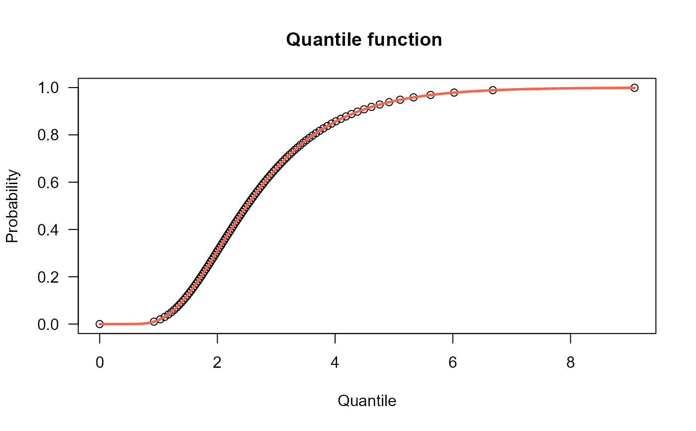
 # Example 3
# The quantile function
p <- seq(from=0, to=0.999, length.out=100)
plot(x=qBS4(p, mu=2, sigma=30), y=p, xlab="Quantile",
las=1, ylab="Probability", main="Quantile function ")
curve(pBS4(x, mu=2, sigma=30),
from=0, add=TRUE, col="tomato", lwd=2.5)
# Example 3
# The quantile function
p <- seq(from=0, to=0.999, length.out=100)
plot(x=qBS4(p, mu=2, sigma=30), y=p, xlab="Quantile",
las=1, ylab="Probability", main="Quantile function ")
curve(pBS4(x, mu=2, sigma=30),
from=0, add=TRUE, col="tomato", lwd=2.5)
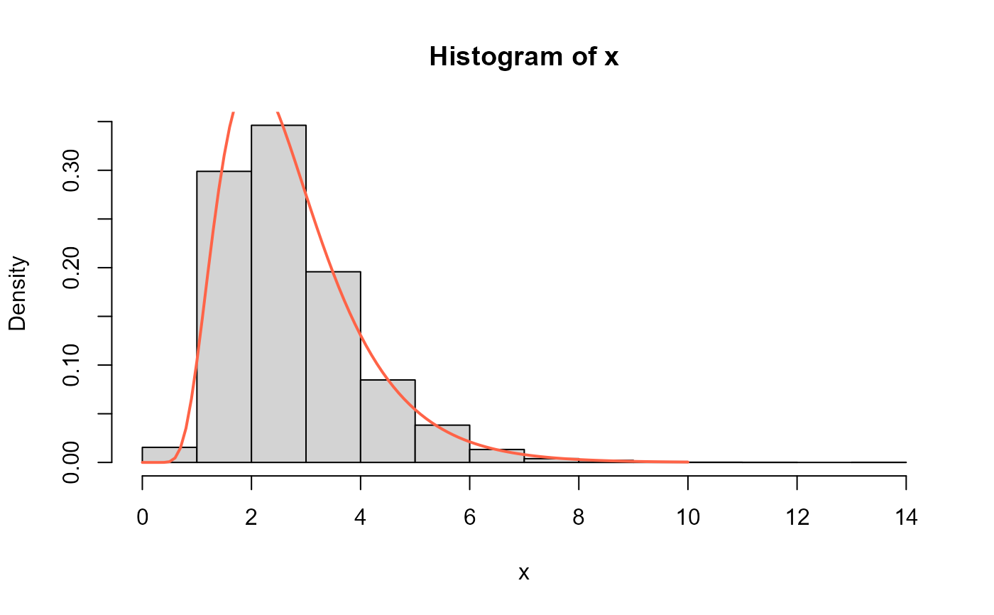
 # Example 4
# The random function
x <- rBS4(n=10000, mu=2, sigma=30)
hist(x, freq=FALSE)
curve(dBS4(x, mu=2, sigma=30), from=0, to=30,
add=TRUE, col="tomato", lwd=2)
# Example 4
# The random function
x <- rBS4(n=10000, mu=2, sigma=30)
hist(x, freq=FALSE)
curve(dBS4(x, mu=2, sigma=30), from=0, to=30,
add=TRUE, col="tomato", lwd=2)
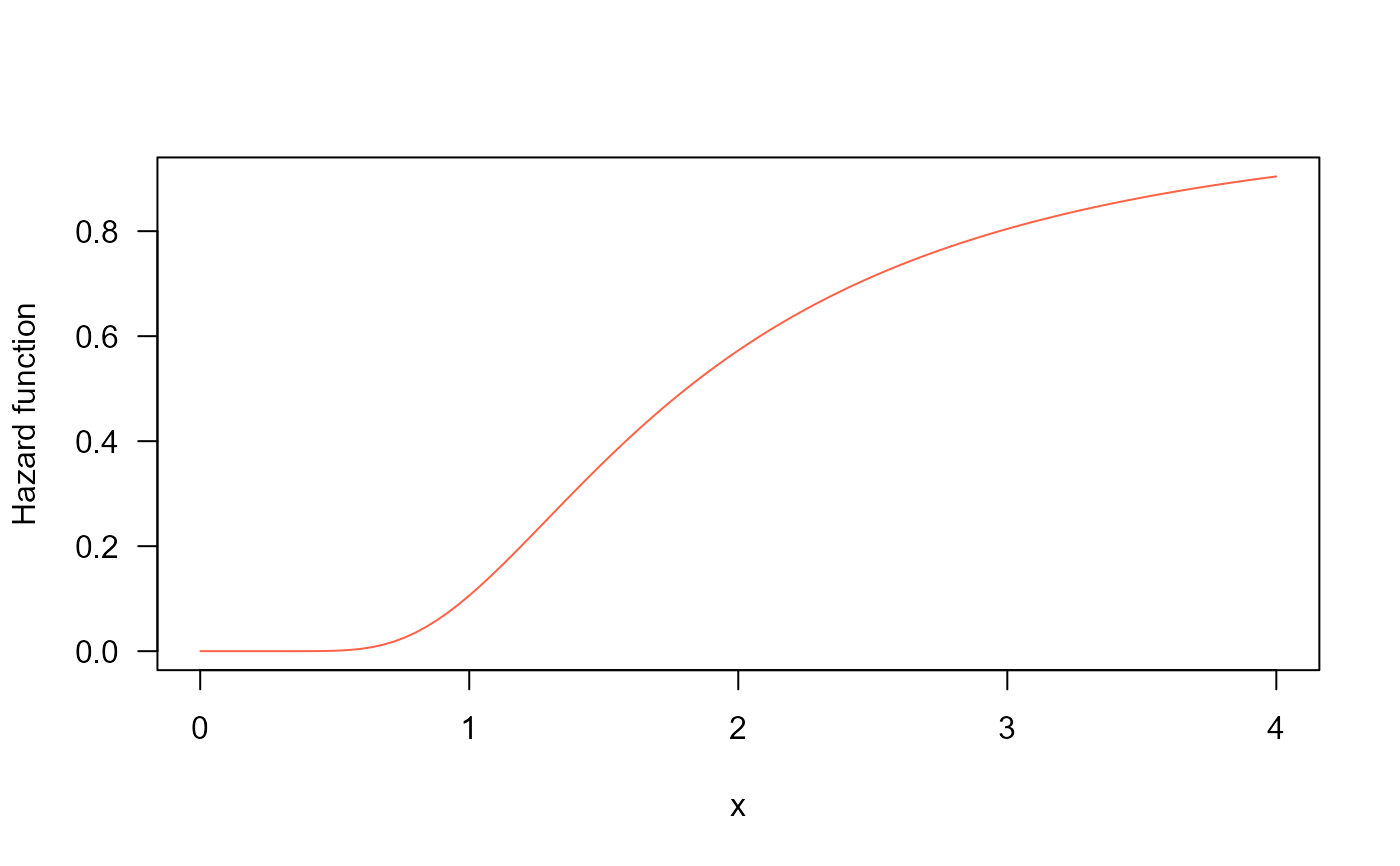
 # Example 5
# The Hazard function
curve(hBS4(x, mu=2, sigma=30), from=0.001, to=40,
col="tomato", ylab="Hazard function", las=1)
# Example 5
# The Hazard function
curve(hBS4(x, mu=2, sigma=30), from=0.001, to=40,
col="tomato", ylab="Hazard function", las=1)