Density, distribution function, quantile function,
random generation and hazard function for the
Birnbaum-Saunders distribution with
parameters mu and sigma.
Usage
dBS2(x, mu = 1, sigma = 1, log = FALSE)

pBS2(q, mu = 1, sigma = 1, lower.tail = TRUE, log.p = FALSE)

qBS2(p, mu = 1, sigma = 1, lower.tail = TRUE, log.p = FALSE)

rBS2(n, mu = 1, sigma = 1)

hBS2(x, mu, sigma)Value
dBS2 gives the density, pBS2 gives the distribution
function, qBS2 gives the quantile function, rBS2
generates random deviates and hBS2 gives the hazard function.
Details
The Birnbaum-Saunders with parameters mu and sigma
has density given by
\(f(x) = \frac{\exp(\sigma/2)\sqrt{\sigma+1}}{4\sqrt{\pi\mu}x^{3/2}} \left[ x + \frac{\mu\sigma}{\sigma+1} \right] \exp\left( \frac{-\sigma}{4} \left(\frac{x(\sigma+1)}{\mu\sigma}+\frac{\mu\sigma}{x(\sigma+1)} \right) \right) \)
for \(x>0\), \(\mu>0\) and \(\sigma>0\). In this parameterization \(E(X)=\mu\) and \(Var(X)=(\mu\sigma)^2(1+5\sigma^2/4)\). The functions proposed here corresponds to the parameterization proposed by Santos-Neto et al. (2014).
References
Santos-Neto, M., Cysneiros, F. J. A., Leiva, V., & Barros, M. (2014). A reparameterized Birnbaum–Saunders distribution and its moments, estimation and applications. REVSTAT-Statistical Journal, 12(3), 247-272.
See also
BS2.
Examples
#Example 1
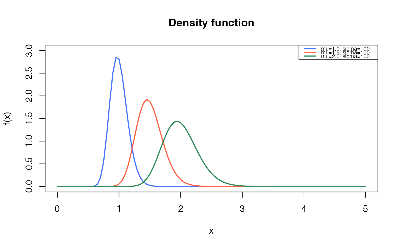
#Plotting the mass function for different parameter values
curve(dBS2(x, mu=1.0, sigma=100),
from=0.001, to=5,
ylim=c(0, 3),
col="royalblue1", lwd=2,
main="Density function",
xlab="x", ylab="f(x)")
curve(dBS2(x, mu=1.5, sigma=100),
col="tomato",
lwd=2,
add=TRUE)
curve(dBS2(x, mu=2.0, sigma=100),
col="seagreen",
lwd=2,
add=TRUE)
legend("topright", legend=c("mu=1.0, sigma=100",
"mu=1.5, sigma=100",
"mu=2.0, sigma=100"),
col=c("royalblue1", "tomato", "seagreen"), lwd=2, cex=0.6)
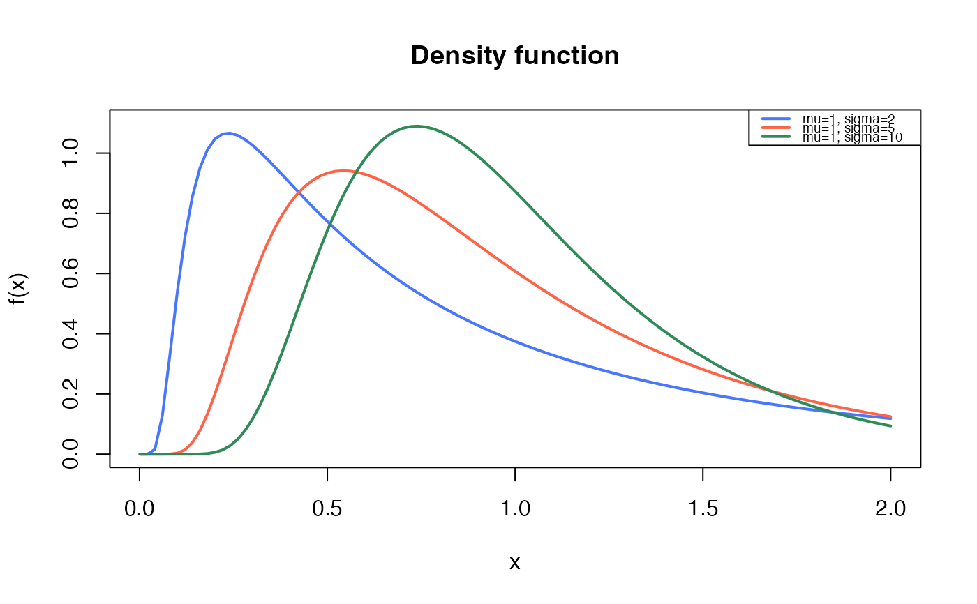
 curve(dBS2(x, mu=1, sigma=2),
from=0.001, to=2,
ylim=c(0, 1.1),
col="royalblue1", lwd=2,
main="Density function",
xlab="x", ylab="f(x)")
curve(dBS2(x, mu=1, sigma=5),
col="tomato",
lwd=2,
add=TRUE)
curve(dBS2(x, mu=1, sigma=10),
col="seagreen",
lwd=2,
add=TRUE)
legend("topright", legend=c("mu=1, sigma=2",
"mu=1, sigma=5",
"mu=1, sigma=10"),
col=c("royalblue1", "tomato", "seagreen"), lwd=2, cex=0.6)
curve(dBS2(x, mu=1, sigma=2),
from=0.001, to=2,
ylim=c(0, 1.1),
col="royalblue1", lwd=2,
main="Density function",
xlab="x", ylab="f(x)")
curve(dBS2(x, mu=1, sigma=5),
col="tomato",
lwd=2,
add=TRUE)
curve(dBS2(x, mu=1, sigma=10),
col="seagreen",
lwd=2,
add=TRUE)
legend("topright", legend=c("mu=1, sigma=2",
"mu=1, sigma=5",
"mu=1, sigma=10"),
col=c("royalblue1", "tomato", "seagreen"), lwd=2, cex=0.6)
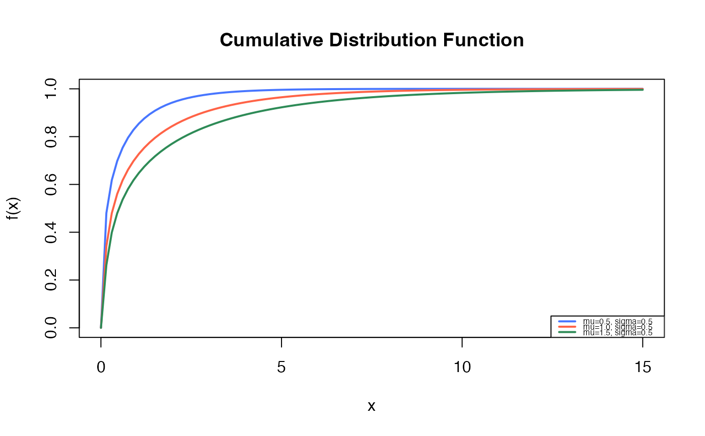
 # Example 2
# Checking if the cumulative curves converge to 1
curve(pBS2(x, mu=0.5, sigma=0.5),
from=0.001, to=15,
ylim=c(0, 1),
col="royalblue1", lwd=2,
main="Cumulative Distribution Function",
xlab="x", ylab="F(x)")
curve(pBS2(x, mu=1, sigma=0.5),
col="tomato",
lwd=2,
add=TRUE)
curve(pBS2(x, mu=1.5, sigma=0.5),
col="seagreen",
lwd=2,
add=TRUE)
legend("bottomright", legend=c("mu=0.5, sigma=0.5",
"mu=1.0, sigma=0.5",
"mu=1.5, sigma=0.5"),
col=c("royalblue1", "tomato", "seagreen"), lwd=2, cex=0.5)
# Example 2
# Checking if the cumulative curves converge to 1
curve(pBS2(x, mu=0.5, sigma=0.5),
from=0.001, to=15,
ylim=c(0, 1),
col="royalblue1", lwd=2,
main="Cumulative Distribution Function",
xlab="x", ylab="F(x)")
curve(pBS2(x, mu=1, sigma=0.5),
col="tomato",
lwd=2,
add=TRUE)
curve(pBS2(x, mu=1.5, sigma=0.5),
col="seagreen",
lwd=2,
add=TRUE)
legend("bottomright", legend=c("mu=0.5, sigma=0.5",
"mu=1.0, sigma=0.5",
"mu=1.5, sigma=0.5"),
col=c("royalblue1", "tomato", "seagreen"), lwd=2, cex=0.5)
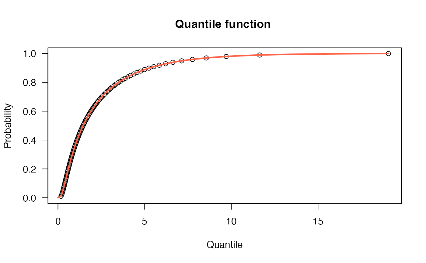
 # Example 3
# The quantile function
p <- seq(from=0, to=0.999, length.out=100)
plot(x=qBS2(p, mu=2.3, sigma=1.7), y=p, xlab="Quantile",
las=1, ylab="Probability", main="Quantile function ")
curve(pBS2(x, mu=2.3, sigma=1.7),
from=0, add=TRUE, col="tomato", lwd=2.5)
# Example 3
# The quantile function
p <- seq(from=0, to=0.999, length.out=100)
plot(x=qBS2(p, mu=2.3, sigma=1.7), y=p, xlab="Quantile",
las=1, ylab="Probability", main="Quantile function ")
curve(pBS2(x, mu=2.3, sigma=1.7),
from=0, add=TRUE, col="tomato", lwd=2.5)
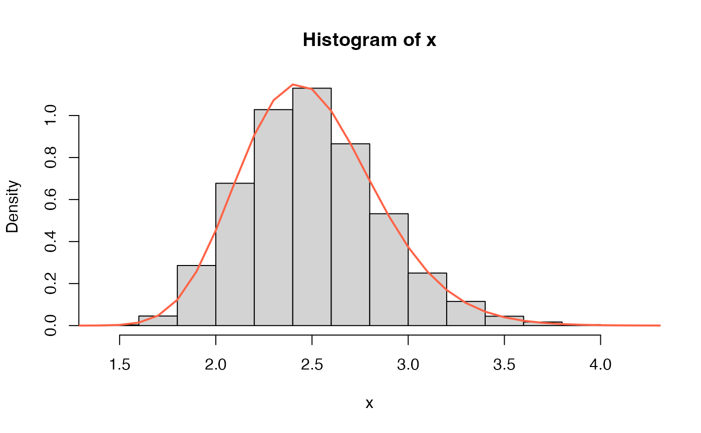
 # Example 4
# The random function
x <- rBS2(n=10000, mu=2.5, sigma=100)
hist(x, freq=FALSE)
curve(dBS2(x, mu=2.5, sigma=100), from=0, to=10,
add=TRUE, col="tomato", lwd=2)
# Example 4
# The random function
x <- rBS2(n=10000, mu=2.5, sigma=100)
hist(x, freq=FALSE)
curve(dBS2(x, mu=2.5, sigma=100), from=0, to=10,
add=TRUE, col="tomato", lwd=2)
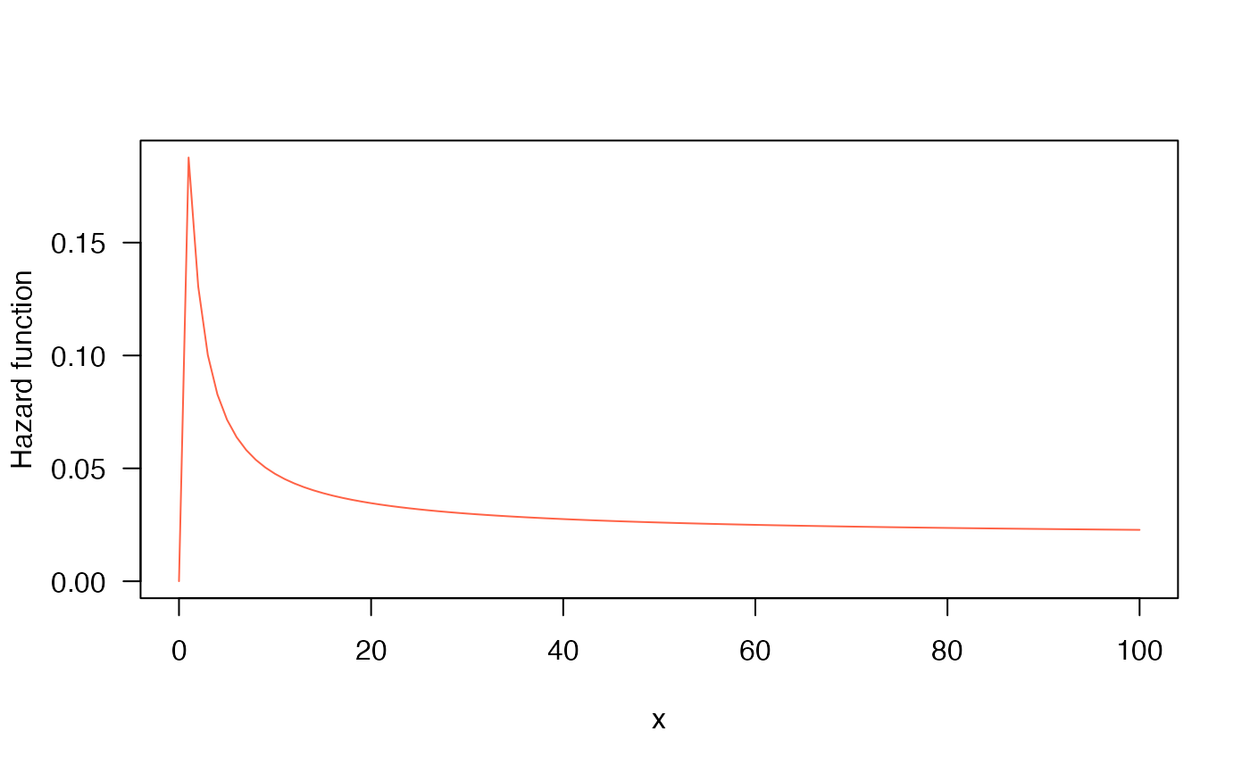
 # Example 5
# The Hazard function
curve(hBS2(x, mu=20, sigma=0.5), from=0.001, to=100,
col="tomato", ylab="Hazard function", las=1)
# Example 5
# The Hazard function
curve(hBS2(x, mu=20, sigma=0.5), from=0.001, to=100,
col="tomato", ylab="Hazard function", las=1)