The Beta Generalized Exponentiated distribution

Density, distribution function, quantile function, random generation and hazard function for the Beta Generalized Exponentiated distribution with parameters mu, sigma, nu and tau.

Usage

dBGE(x, mu, sigma, nu, tau, log = FALSE)

pBGE(q, mu, sigma, nu, tau, lower.tail = TRUE, log.p = FALSE)

qBGE(p, mu, sigma, nu, tau, lower.tail = TRUE, log.p = FALSE)

rBGE(n, mu, sigma, nu, tau)

hBGE(x, mu, sigma, nu, tau)

Arguments

x, q: vector of quantiles.
mu: parameter.
sigma: parameter.
nu: parameter.
tau: parameter.
log, log.p: logical; if TRUE, probabilities p are given as log(p).
lower.tail: logical; if TRUE (default), probabilities are P[X <= x], otherwise, P[X > x].
p: vector of probabilities.
n: number of observations.

Value

dBGE gives the density, pBGE gives the distribution function, qBGE gives the quantile function, rBGE generates random deviates and hBGE gives the hazard function.

Details

The Beta Generalized Exponentiated Distribution with parameters mu, sigma, nu and tau has density given by

\(f(x)= \frac{\nu \tau}{B(\mu, \sigma)} \exp(-\nu x)(1- \exp(-\nu x))^{\tau \mu - 1} (1 - (1- \exp(-\nu x))^\tau)^{\sigma -1},\)

for \(x > 0\), \(\mu > 0\), \(\sigma > 0\), \(\nu > 0\) and \(\tau > 0\).

References

Almalki, S. J., & Nadarajah, S. (2014). Modifications of the Weibull distribution: A review. Reliability Engineering & System Safety, 124, 32-55.

Barreto-Souza, W., Santos, A. H., & Cordeiro, G. M. (2010). The beta generalized exponential distribution. Journal of statistical Computation and Simulation, 80(2), 159-172.

Author

Johan David Marin Benjumea, johand.marin@udea.edu.co

Examples

old_par <- par(mfrow = c(1, 1)) # save previous graphical parameters

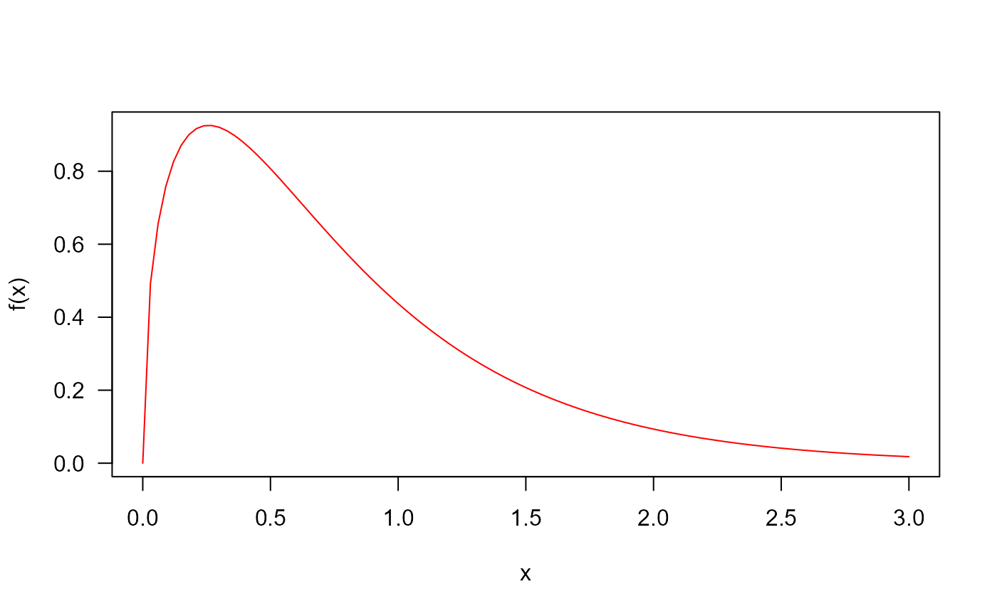
## The probability density function 
curve(dBGE(x, mu = 1.5, sigma =1.7, nu=1, tau=1), from = 0, to = 3, 
      col = "red", las = 1, ylab = "f(x)")


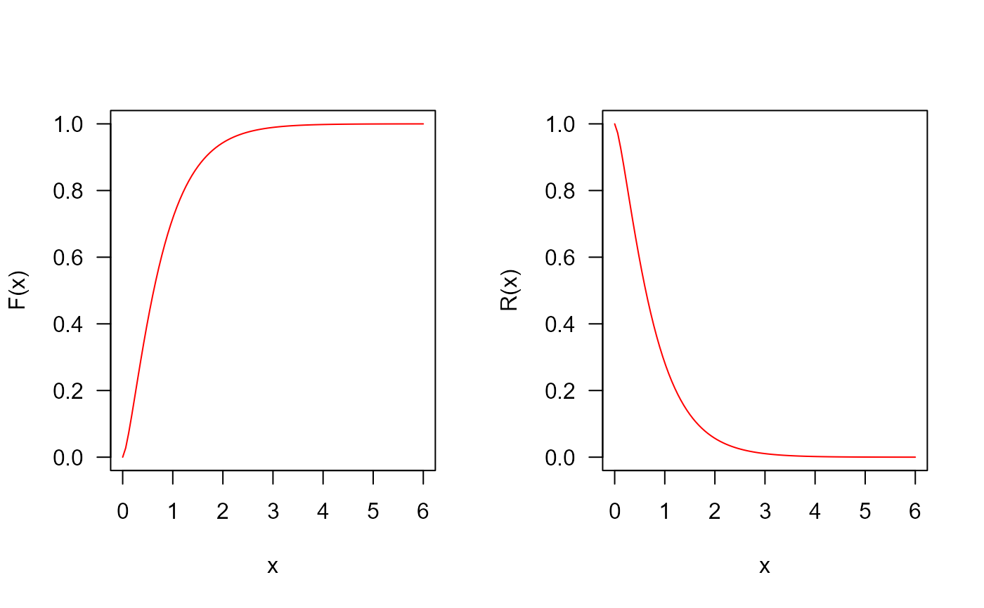
## The cumulative distribution and the Reliability function
par(mfrow = c(1, 2))
curve(pBGE(x, mu = 1.5, sigma =1.7, nu=1, tau=1), from = 0, to = 6, 
      ylim = c(0, 1), col = "red", las = 1, ylab = "F(x)")
curve(pBGE(x, mu = 1.5, sigma =1.7, nu=1, tau=1, lower.tail = FALSE), 
      from = 0, to = 6, ylim = c(0, 1), col = "red", las = 1, ylab = "R(x)")


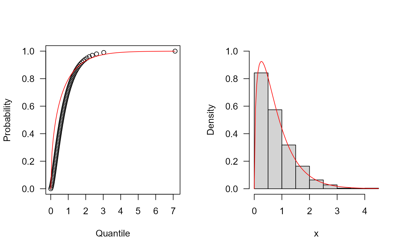
## The quantile function
p <- seq(from = 0, to = 0.99999, length.out = 100)
plot(x = qBGE(p = p, mu = 1.5, sigma =1.7, nu=1, tau=1), y = p, 
     xlab = "Quantile", las = 1, ylab = "Probability")
curve(pBGE(x, mu = (1/4), sigma =1, nu=1, tau=2), from = 0, add = TRUE, 
      col = "red")

## The random function
hist(rBGE(1000, mu = 1.5, sigma =1.7, nu=1, tau=1), freq = FALSE, xlab = "x", 
     ylim = c(0, 1), las = 1, main = "")
curve(dBGE(x, mu = 1.5, sigma =1.7, nu=1, tau=1),  from = 0, add = TRUE, 
      col = "red", ylim = c(0, 0.5))


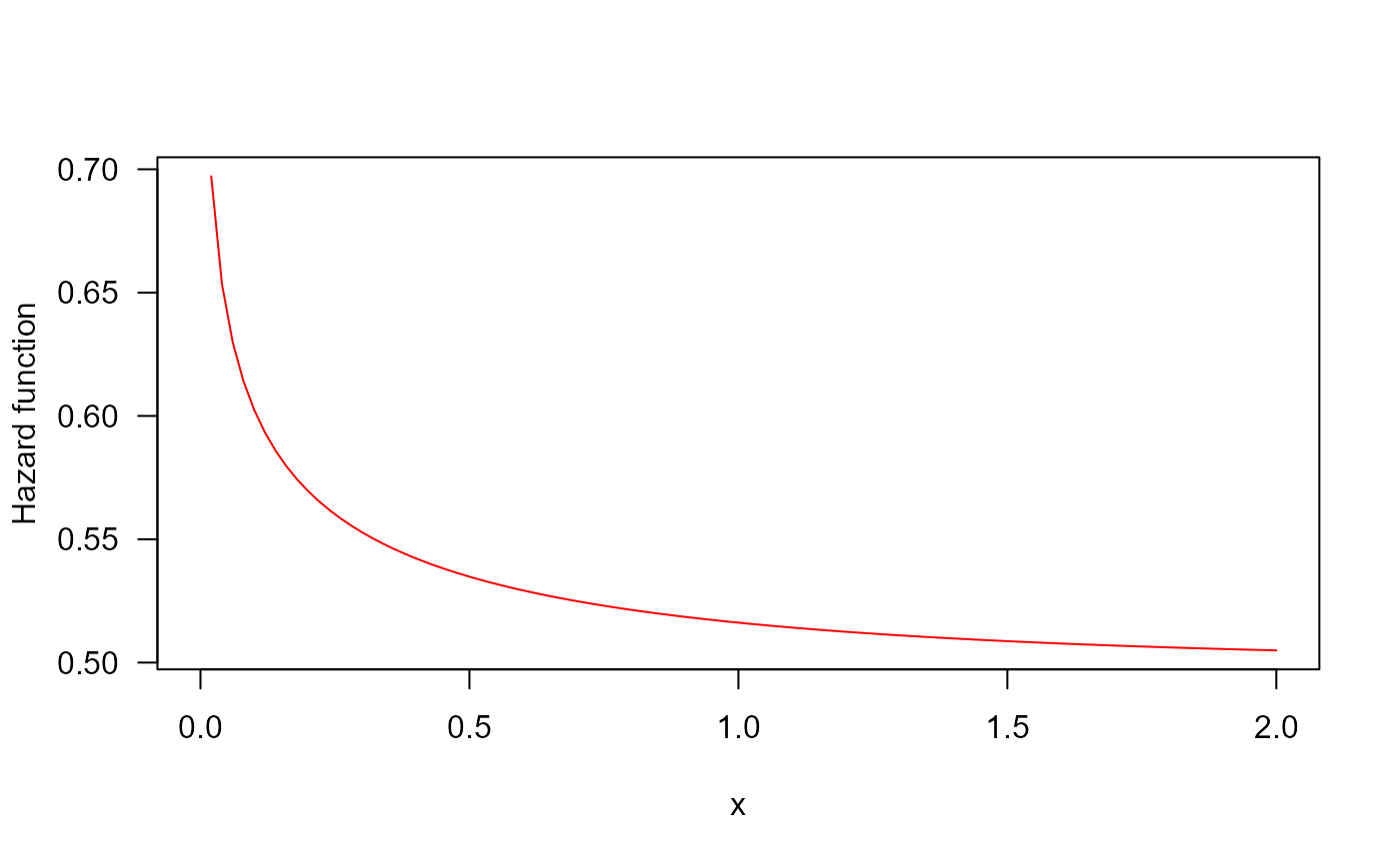
## The Hazard function(
par(mfrow=c(1,1))
curve(hBGE(x, mu = 0.9, sigma =0.5, nu=1, tau=1), from = 0, to = 2, 
      col = "red", ylab = "Hazard function", las = 1)


par(old_par) # restore previous graphical parameters