Zero Inflated Bivariate Poisson Distribution - Laksh

This function obtains the probability for the Zero Inflated Bivariate Poisson distribution under the parameterization of Lakshminarayana et. al (1993).

dZIBP_Laksh(x, l1, l2, alpha, psi, log = FALSE)

rZIBP_Laksh(n, l1, l2, alpha, psi, max_val_x1 = NULL, max_val_x2 = NULL)

Arguments

x

vector or matrix of quantiles. When x is a matrix, each row is taken to be a quantile and columns correspond to the number of dimensions p.

l1

mean for the marginal \(X_1\) variable with Poisson distribution.

l2

mean for the marginal \(X_2\) variable with Poisson distribution.

alpha

third parameter.

psi

parameter with the contamination proportion, \(0 \leq \psi \leq 1\).

log

logical; if TRUE, densities d are given as log(d).

n

number of random observations.

max_val_x1

maximum value for \(X_1\) that is expected, by default it is 100.

max_val_x2

maximum value for \(X_2\) that is expected, by default it is 100.

Value

Returns the density for a given data x.

References

Lakshminarayana, J., Pandit, S. N., & Srinivasa Rao, K. (1999). On a bivariate Poisson distribution. Communications in Statistics-Theory and Methods, 28(2), 267-276.

Author

Freddy Hernandez-Barajas, fhernanb@unal.edu.co

Examples

# Example 1 ---------------------------------------------------------------
# Probability for single values of X1 and X2
dZIBP_Laksh(c(0, 0), l1=3, l2=4, alpha=1, psi=0.15)
#> [1] 0.1513813
dZIBP_Laksh(c(1, 0), l1=3, l2=4, alpha=1, psi=0.15)
#> [1] 0.002791271
dZIBP_Laksh(c(0, 1), l1=3, l2=4, alpha=1, psi=0.15)
#> [1] 0.003859537

# Probability for a matrix the values of X1 and X2
x <- matrix(c(0, 0,
              1, 0,
              0, 1), ncol=2, byrow=TRUE)
x
#>      [,1] [,2]
#> [1,]    0    0
#> [2,]    1    0
#> [3,]    0    1
dZIBP_Laksh(x=x, l1=3, l2=4, alpha=1, psi=0.15)
#> [1] 0.151381291 0.002791271 0.003859537

# Checking if the probabilities sum 1
val_x1 <- val_x2 <- 0:50
space <- expand.grid(val_x1, val_x2)
space <- as.matrix(space)

l1 <- 3
l2 <- 4
alpha <- -1.27
psi <- 0.15

probs <- dZIBP_Laksh(x=space, l1=l1, l2=l2, alpha=alpha, psi=psi)
sum(probs)
#> [1] 1

# Example 2 ---------------------------------------------------------------
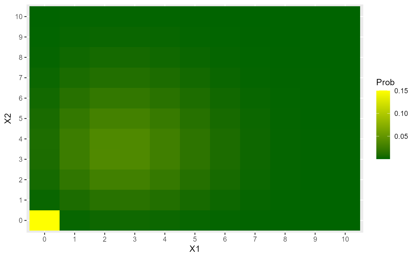
# Heat map for a ZIBP_Laksh

l1 <- 3
l2 <- 4
alpha <- -1.2
psi <- 0.15

X1 <- 0:10
X2 <- 0:10
data <- expand.grid(X1=X1, X2=X2)
data$Prob <- dZIBP_Laksh(x=data, l1=l1, l2=l2, alpha=alpha, psi=psi)
data$X1 <- factor(data$X1)
data$X2 <- factor(data$X2)

library(ggplot2)
ggplot(data, aes(X1, X2, fill=Prob)) +
  geom_tile() +
  scale_fill_gradient(low="darkgreen", high="yellow")



# Example 3 ---------------------------------------------------------------
# Generating random values and moment estimations

l1 <- 15
l2 <- 13
correct_alpha_BP_Laksh(l1, l2)
#> $min_alpha
#> [1] -1.000346
#> 
#> $max_alpha
#> [1] 1.000346
#> 
alpha <- 0.9
psi <- 0.20

x <- rZIBP_Laksh(n=50000, l1, l2, alpha, psi)
moments_estim_ZIBP_Laksh(x)
#>    l1_hat    l2_hat alpha_hat   psi_hat 
#>   14.9985   13.0044   -1.0003    0.2006 

# Example 4 ---------------------------------------------------------------
# Estimating the parameters using the loglik function

# Loglik function
llZIBP_Laksh <- function(param, x) {
  l1    <- param[1]  # param: is the parameter vector
  l2    <- param[2]
  alpha <- param[3]
  psi   <- param[4]
  sum(dZIBP_Laksh(x=x, l1=l1, l2=l2,
                  alpha=alpha, psi=psi, log=TRUE))
}

# The known parameters
l1 <- 5
l2 <- 3
correct_alpha_BP_Laksh(l1=l1, l2=l2)
#> $min_alpha
#> [1] -1.228726
#> 
#> $max_alpha
#> [1] 1.228726
#> 
alpha <- -1.20
psi <- 0.20

set.seed(12345)
x <- rZIBP_Laksh(n=500, l1=l1, l2=l2, alpha=alpha, psi=psi)

# To obtain reasonable values for alpha
theta <- as.numeric(moments_estim_ZIBP_Laksh(x))
theta
#> [1]  5.1505  2.8738 -1.2420  0.1760

# To create start parameters
min_alpha <- correct_alpha_BP_Laksh(l1=theta[1],
                                    l2=theta[2])$min_alpha
max_alpha <- correct_alpha_BP_Laksh(l1=theta[1],
                                    l2=theta[2])$max_alpha

start_param <- theta
names(start_param) <- c("l1_hat", "l2_hat", "alpha_hat", "psi_hat")
start_param
#>    l1_hat    l2_hat alpha_hat   psi_hat 
#>    5.1505    2.8738   -1.2420    0.1760 

# Estimating parameters
res1 <- optim(fn = llZIBP_Laksh,
              par = start_param,
              lower = c(0.001, 0.001, min_alpha, 0.0001),
              upper = c(  Inf,   Inf, max_alpha, 0.9999),
              method = "L-BFGS-B",
              control = list(maxit=100000, fnscale=-1),
              x=x)

res1
#> $par
#>     l1_hat     l2_hat  alpha_hat    psi_hat 
#>  5.1490422  2.8716417 -1.2420012  0.1759906 
#> 
#> $value
#> [1] -1960.879
#> 
#> $counts
#> function gradient 
#>        6        6 
#> 
#> $convergence
#> [1] 0
#> 
#> $message
#> [1] "CONVERGENCE: REL_REDUCTION_OF_F <= FACTR*EPSMCH"
#>