This function obtains the probability for the Zero Inflated Bivariate Poisson distribution under the parameterization of Kouakou et. al (2021).
dZIBP_HOL(x, l1, l2, l0, psi, log = FALSE)

rZIBP_HOL(n, l1, l2, l0, psi)
Arguments
- x
vector or matrix of quantiles. When
xis a matrix, each row is taken to be a quantile and columns correspond to the number of dimensionsp.- l1
mean for \(Z_1\) variable with Poisson distribution.
- l2
mean for \(Z_2\) variable with Poisson distribution.
- l0
mean for \(U\) variable with Poisson distribution.
- psi
parameter with the contamination proportion, \(0 \leq \psi \leq 1\).
- log
logical; if
TRUE, densities d are given as log(d).- n
number of random observations.
Value
Returns the density for a given data x.
References
P. Holgate. Estimation for the bivariate poisson distribution. Biometrika, 51(1/2):241–245, 1964. ISSN 00063444, 14643510. URL http://www.jstor.org/stable/2334210.
Konan Jean Geoffroy Kouakou, Ouagnina Hili, and Jean-Francois Dupuy. Estimation in the zero-inflated bivariate poisson model with an application to health-care utilization data. Afrika Statistika, 16(2):2767–2788, 2021.
Examples
# Example 1 ---------------------------------------------------------------
# Probability for single values of X1 and X2
dZIBP_HOL(c(0, 0), l1=3, l2=4, l0=1, psi=0.15)
#> [1] 0.1502851
dZIBP_HOL(c(1, 0), l1=3, l2=4, l0=1, psi=0.15)
#> [1] 0.0008554297
dZIBP_HOL(c(0, 1), l1=3, l2=4, l0=1, psi=0.15)
#> [1] 0.001140573
# Probability for a matrix the values of X1 and X2
x <- matrix(c(0, 0,
1, 0,
0, 1), ncol=2, byrow=TRUE)
x
#> [,1] [,2]
#> [1,] 0 0
#> [2,] 1 0
#> [3,] 0 1
dZIBP_HOL(x=x, l1=3, l2=4, l0=1, psi=0.15)
#> [1] 0.1502851432 0.0008554297 0.0011405729
# Checking if the probabilities sum 1
val_x1 <- val_x2 <- 0:50
space <- expand.grid(val_x1, val_x2)
space <- as.matrix(space)
l1 <- 3
l2 <- 4
l0 <- 1.27
psi <- 0.15
probs <- dZIBP_HOL(x=space, l1=l1, l2=l2, l0=l0, psi=psi)
sum(probs)
#> [1] 1
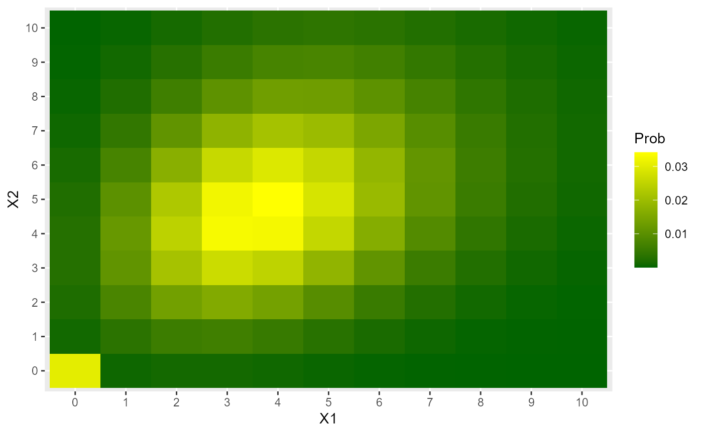
# Example 2 ---------------------------------------------------------------
# Heat map for a ZIBP_HOL
l1 <- 3
l2 <- 4
l0 <- 1.2
psi <- 0.03
X1 <- 0:10
X2 <- 0:10
data <- expand.grid(X1=X1, X2=X2)
data$Prob <- dZIBP_HOL(x=data, l1=l1, l2=l2, l0=l0, psi=psi)
data$X1 <- factor(data$X1)
data$X2 <- factor(data$X2)
library(ggplot2)
ggplot(data, aes(X1, X2, fill=Prob)) +
geom_tile() +
scale_fill_gradient(low="darkgreen", high="yellow")
 # Example 3 ---------------------------------------------------------------
# Generating random values and moment estimations
l1 <- 13
l2 <- 8
l0 <- 5
psi <- 0.15
x <- rZIBP_HOL(n=500, l1, l2, l0, psi)
moments_estim_ZIBP_HOL(x)
#> l1_hat l2_hat l0_hat psi_hat
#> 13.357003 8.242515 4.769214 0.136058
# Example 4 ---------------------------------------------------------------
# Estimating the parameters using the loglik function
# Loglik function
llZIBP_HOL <- function(param, x) {
l1 <- param[1] # param: is the parameter vector
l2 <- param[2]
l0 <- param[3]
psi <- param[4]
sum(dZIBP_HOL(x=x, l1=l1, l2=l2,
l0=l0, psi=psi, log=TRUE))
}
# The known parameters
l1 <- 5
l2 <- 3
psi <- 0.20
l0 <- 1.20
set.seed(12345)
x <- rZIBP_HOL(n=500, l1=l1, l2=l2, l0=l0, psi=psi)
# To obtain reasonable values for l0
start_param <- moments_estim_ZIBP_HOL(x)
start_param
#> l1_hat l2_hat l0_hat psi_hat
#> 4.8858732 3.3560129 1.1656262 0.2114351
# Estimating parameters
res1 <- optim(fn = llZIBP_HOL,
par = start_param,
lower = c(0.001, 0.001, 0.001, 0.0001),
upper = c( Inf, Inf, Inf, 0.9999),
method = "L-BFGS-B",
control = list(maxit=100000, fnscale=-1),
x=x)
res1
#> $par
#> l1_hat l2_hat l0_hat psi_hat
#> 4.7252011 2.8382652 1.3919600 0.2199004
#>
#> $value
#> [1] -1967.426
#>
#> $counts
#> function gradient
#> 17 17
#>
#> $convergence
#> [1] 0
#>
#> $message
#> [1] "CONVERGENCE: REL_REDUCTION_OF_F <= FACTR*EPSMCH"
#>
# Example 3 ---------------------------------------------------------------
# Generating random values and moment estimations
l1 <- 13
l2 <- 8
l0 <- 5
psi <- 0.15
x <- rZIBP_HOL(n=500, l1, l2, l0, psi)
moments_estim_ZIBP_HOL(x)
#> l1_hat l2_hat l0_hat psi_hat
#> 13.357003 8.242515 4.769214 0.136058
# Example 4 ---------------------------------------------------------------
# Estimating the parameters using the loglik function
# Loglik function
llZIBP_HOL <- function(param, x) {
l1 <- param[1] # param: is the parameter vector
l2 <- param[2]
l0 <- param[3]
psi <- param[4]
sum(dZIBP_HOL(x=x, l1=l1, l2=l2,
l0=l0, psi=psi, log=TRUE))
}
# The known parameters
l1 <- 5
l2 <- 3
psi <- 0.20
l0 <- 1.20
set.seed(12345)
x <- rZIBP_HOL(n=500, l1=l1, l2=l2, l0=l0, psi=psi)
# To obtain reasonable values for l0
start_param <- moments_estim_ZIBP_HOL(x)
start_param
#> l1_hat l2_hat l0_hat psi_hat
#> 4.8858732 3.3560129 1.1656262 0.2114351
# Estimating parameters
res1 <- optim(fn = llZIBP_HOL,
par = start_param,
lower = c(0.001, 0.001, 0.001, 0.0001),
upper = c( Inf, Inf, Inf, 0.9999),
method = "L-BFGS-B",
control = list(maxit=100000, fnscale=-1),
x=x)
res1
#> $par
#> l1_hat l2_hat l0_hat psi_hat
#> 4.7252011 2.8382652 1.3919600 0.2199004
#>
#> $value
#> [1] -1967.426
#>
#> $counts
#> function gradient
#> 17 17
#>
#> $convergence
#> [1] 0
#>
#> $message
#> [1] "CONVERGENCE: REL_REDUCTION_OF_F <= FACTR*EPSMCH"
#>