Bivariate Poisson Distribution - Holgate

This function obtains the probability for the Bivariate Poisson distribution under the parameterization of Holgate et. al (1964).

dBP_HOL(x, l1, l2, l0, log = FALSE)

rBP_HOL(n, l1, l2, l0)

Arguments

x

vector or matrix of quantiles. When x is a matrix, each row is taken to be a quantile and columns correspond to the number of dimensions p.

l1

mean for \(Z_1\) variable with Poisson distribution.

l2

mean for \(Z_2\) variable with Poisson distribution.

l0

mean for \(U\) variable with Poisson distribution.

log

logical; if TRUE, densities d are given as log(d).

n

number of random observations.

Value

Returns the density for a given data x.

References

P. Holgate. Estimation for the bivariate poisson distribution. Biometrika, 51(1/2):241–245, 1964. ISSN 00063444, 14643510. URL http://www.jstor.org/stable/2334210.

Author

Freddy Hernandez-Barajas, fhernanb@unal.edu.co

Examples

# Example 1 ---------------------------------------------------------------
# Probability for single values of X1 and X2
dBP_HOL(c(0, 0), l1=3, l2=4, l0=1)
#> [1] 0.0003354626
dBP_HOL(c(1, 0), l1=3, l2=4, l0=1)
#> [1] 0.001006388
dBP_HOL(c(0, 1), l1=3, l2=4, l0=1)
#> [1] 0.001341851

# Probability for a matrix the values of X1 and X2
x <- matrix(c(0, 0,
              1, 0,
              0, 1), ncol=2, byrow=TRUE)
x
#>      [,1] [,2]
#> [1,]    0    0
#> [2,]    1    0
#> [3,]    0    1
dBP_HOL(x=x, l1=3, l2=4, l0=1)
#> [1] 0.0003354626 0.0010063879 0.0013418505

# Checking if the probabilities sum 1
val_x1 <- val_x2 <- 0:50
space <- expand.grid(val_x1, val_x2)
space <- as.matrix(space)

l1 <- 3
l2 <- 4
l0 <- 5

probs <- dBP_HOL(x=space, l1=l1, l2=l2, l0=l0)
sum(probs)
#> [1] 1

# Example 2 ---------------------------------------------------------------
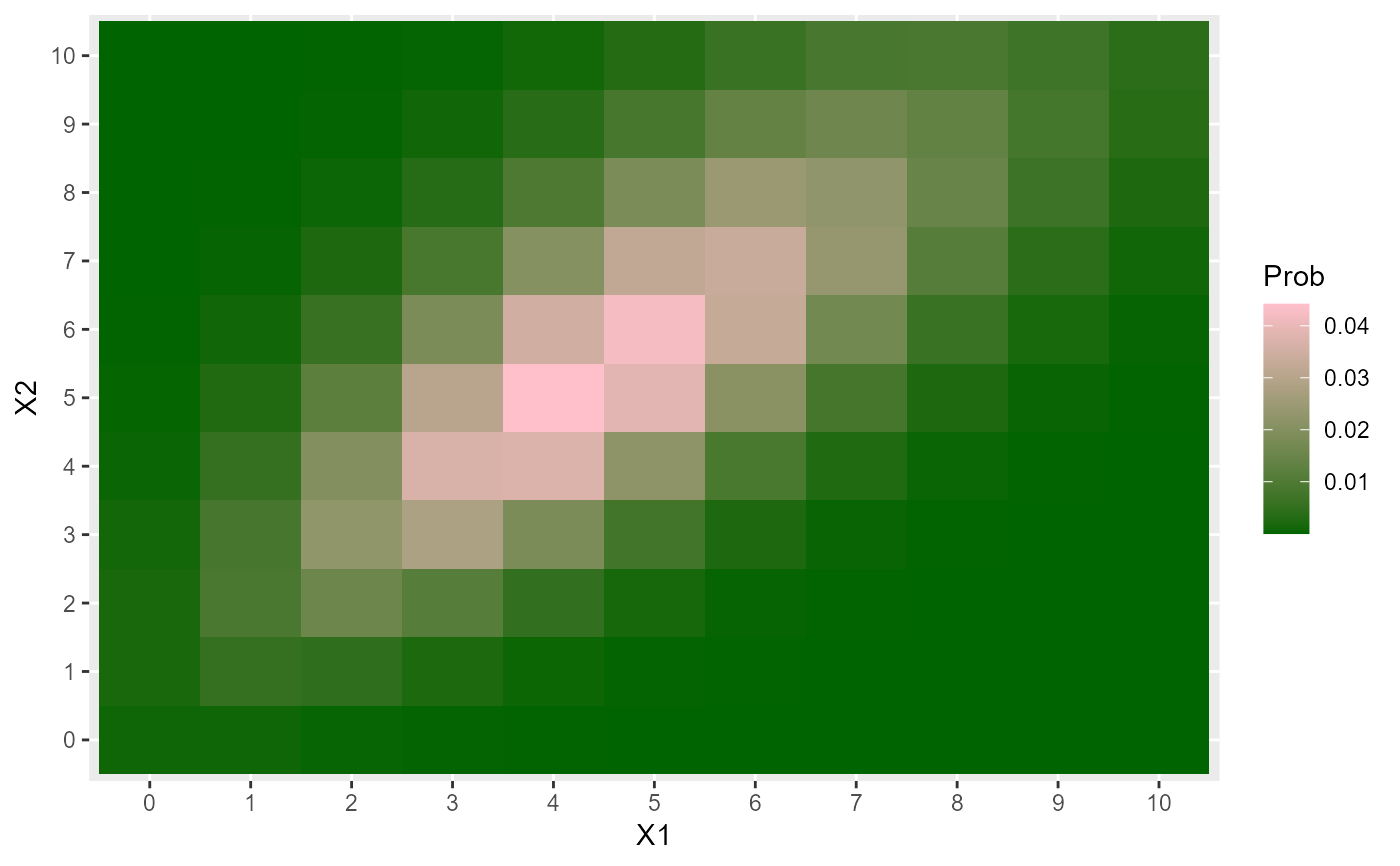
# Heat map for a BP_HOL

l1 <- 1
l2 <- 2
l0 <- 4

X1 <- 0:10
X2 <- 0:10
data <- expand.grid(X1=X1, X2=X2)
data$Prob <- dBP_HOL(x=data, l1=l1, l2=l2, l0=l0)
data$X1 <- factor(data$X1)
data$X2 <- factor(data$X2)

library(ggplot2)
ggplot(data, aes(X1, X2, fill=Prob)) +
  geom_tile() +
  scale_fill_gradient(low="darkgreen", high="pink")


# Example 3 ---------------------------------------------------------------
# Generating random values and moment estimations

l1 <- 1
l2 <- 2
l0 <- 4

x <- rBP_HOL(n=500, l1, l2, l0)
moments_estim_BP_HOL(x)
#>   l1_hat   l2_hat   l0_hat 
#> 1.453739 2.361739 3.522261 

# Example 4 ---------------------------------------------------------------
# Estimating the parameters using the loglik function

# Loglik function
llBP_HOL <- function(param, x) {
  l1 <- param[1]  # param: is the parameter vector
  l2 <- param[2]
  l0 <- param[3]
  sum(dBP_HOL(x=x, l1=l1, l2=l2, l0=l0, log=TRUE))
}

# The known parameters
l1 <- 1
l2 <- 2
l0 <- 4

set.seed(12345)
x <- rBP_HOL(n=500, l1=l1, l2=l2, l0=l0)

# To obtain reasonable values for l0
start_param <- moments_estim_BP_HOL(x)
start_param
#>    l1_hat    l2_hat    l0_hat 
#> 0.7746052 1.6526052 4.4573948 

# Estimating parameters
res1 <- optim(fn = llBP_HOL,
              par = start_param,
              lower = c(0.001, 0.001, 0.001),
              upper = c(  Inf,   Inf,   Inf),
              method = "L-BFGS-B",
              control = list(maxit=100000, fnscale=-1),
              x=x)

res1
#> $par
#>    l1_hat    l2_hat    l0_hat 
#> 0.8505074 1.7285063 4.3814917 
#> 
#> $value
#> [1] -2043.163
#> 
#> $counts
#> function gradient 
#>        9        9 
#> 
#> $convergence
#> [1] 0
#> 
#> $message
#> [1] "CONVERGENCE: REL_REDUCTION_OF_F <= FACTR*EPSMCH"
#>